2Functions, Graphs, and Just Enough Algebra

Before calculus asks you to do anything hard, it quietly assumes you are comfortable with a few small things. Not many, and not deep — but if any of them feel shaky, every later chapter feels shaky too, and that is usually what "I'm bad at math" turns out to mean. So this chapter is a refresher, and it is meant to feel like relief, not a test. We will look at exactly three things calculus leans on: a function (a rule that turns one number into another), the graph of a function (a picture of that rule), and the slope of a line (a single number for "how steep"). That is the whole toolkit. If you already know this, you will move fast; if you don't, we start from the ground and assume nothing.

2.1A function is a machine

Here is the single most useful way to picture a function. A function is a machine: you drop a number in, it does one fixed thing to it, and one number comes out. Same input, same output, every time — that is the whole promise a function makes.

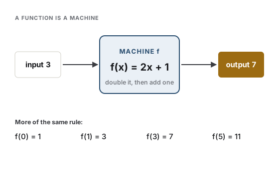
The machine in the picture doubles its input and adds one. Feed it \(3\) and it hands back \(7\). Feed it \(0\) and you get \(1\); feed it \(5\) and you get \(11\). Nothing surprising — but notice the discipline of it. The machine never gets to pick; the rule decides. And it always returns exactly one output, never two. That "exactly one" is the fine print that makes a function a function, and later it is what lets us talk about the slope at a point instead of a fistful of them.

Now the notation, which is genuinely the scariest-looking part of all of this and genuinely the least deep. We give the machine a name — usually \(f\) — and we write \(f(3) = 7\) to mean "feed \(3\) into the machine \(f\), and \(7\) comes out." That is all \(f(3)\) ever means: the output when the input is \(3\). This is function notation, the shorthand \(f(x)\) for "the output of the machine \(f\) when you feed it \(x\)."

To capture the whole machine in one line, we use a placeholder \(x\) standing for "whatever you feed in" and write the rule once:

Read that as a recipe, left to right: take your input \(x\), double it, add one, and that is the output. The \(x\) is not a specific number and it is not a mystery to solve for — it is just a name for the empty slot. Swap in a real number and the machine runs: \(f(3) = 2 \cdot 3 + 1 = 7\).

2.2The graph is a picture of every pair at once

Listing input-output pairs works, but your eye is far better at pictures than at tables. So we draw the function. The graph of a function is the picture you get by treating each input-output pair as a point — the input measured left-to-right, the output measured up-and-down — and plotting all of them at once.

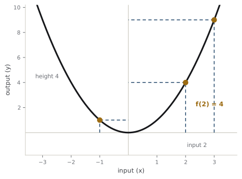
The convention is worth saying plainly, because it never changes: the input goes on the horizontal direction, the output on the vertical. People call the horizontal one the \(x\)-axis and the vertical one the \(y\)-axis, and they often write \(y = f(x)\) to mean "the height \(y\) is the output of \(f\) at the input \(x\)." So a point on the graph is a pair "(input, height)," and to read the graph you go up from an input until you hit the curve, then across to read off the height. In the picture, the input \(2\) sends you up to the curve and across to height \(4\), so \(f(2) = 4\) for this particular machine, which squares its input.

Why does this matter for calculus? Because every big idea ahead is really a question about the shape of a graph. Where is it climbing and where is it falling? How steep is it right here? How much area sits underneath it? You will reason about those by looking at curves, and the whole point of a graph is that it turns a rule you have to compute into a shape you can just see.

2.3Lines, slope, and just enough algebra

Of all the shapes a graph can take, the straight line is the one calculus cares about most — not because lines are exciting, but because the entire subject is built on approximating curvy things by straight ones. So we need one number that captures a line completely: its steepness.

Picture walking up a ramp from left to right. Two things describe your climb: how far you move across, and how far you rise up over that span. The slope is the second divided by the first — the rise divided by the run — the amount you climb for each step you take sideways.

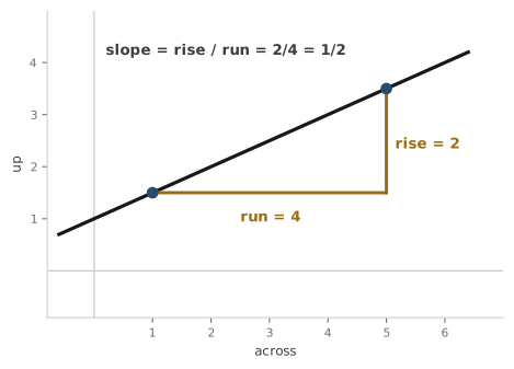
Pick any two points on the line. Measure how far you go across between them — the run — and how far up — the rise — and divide:

The magic of a straight line is that this ratio is the same no matter which two points you choose. Steeper lines give bigger slopes; a line going downhill has a negative slope; a flat line has slope zero.

A line with a fixed slope is called a linear function, and it has a tidy standard form. If a line has slope \(m\) and crosses the vertical axis at height \(b\) — that crossing height is the y-intercept, the output when the input is \(0\) — then its rule is

You have already met one: \(f(x) = 2x + 1\) from the first section is a line of slope \(2\) and \(y\)-intercept \(1\). Here \(m\) is exactly the rise-over-run steepness, and \(b\) just slides the whole line up or down.

Now, the reason slope earns a whole section in a calculus book. A curve does not have one slope — it bends, so its steepness keeps changing. But if you zoom way in on any smooth curve, a tiny piece of it looks nearly straight, and that little straight piece has a slope you can measure. The derivative, the star of Part II, is exactly this: the slope of a curve at a single point, found by measuring rise over run on shorter and shorter straight pieces until the answer settles. Everything you just refreshed about lines is the ground that idea stands on.

Two small algebra moves round out the "just enough," because later chapters use them without pausing. The first is rearranging an equation: doing the same thing to both sides to isolate what you want. If \(y = 2x + 1\) and you would rather have \(x\) in terms of \(y\), subtract \(1\) from both sides and divide by \(2\): \(x = (y - 1)/2\). Nothing changes about the relationship; you have just solved for the other letter.

The second is factoring: rewriting a sum as a product, which is how you find where an expression equals zero and how you cancel a troublesome term. The pattern you will see most is the difference of two squares,

which you can check by multiplying the right side back out. This exact move is what rescues the derivative from dividing by zero. When you compute a slope over a tiny run and get something like \(\frac{x^2 - 1}{x - 1}\), factoring the top lets you cancel the \(x - 1\) and escape the \(\frac{0}{0}\) trap — you'll watch it happen in Chapter 3 and again in Chapter 5.

None of this is calculus yet. It is the floor calculus stands on, and now it is solid. When the next chapters say "the slope of the curve" or "solve for \(x\)" or "factor and cancel," you will not have to stop and worry — you have already done it here.