5Genetics for the ML Practitioner

The molecules in Part II came with a ground truth you could, in principle, measure: a structure is right or wrong, a binding affinity is a number you can put on a plate. Genetics hands you something looser. Genetic variation is nature's own perturbation experiment run across billions of people, and it is the closest thing biology has to a randomized trial. But three things sit between a statistical signal and a mechanism, and each one trips up practitioners who treat a genotype table like any other feature matrix. Evolution has shaped which variants exist and at what frequency. Nearby variants travel together and smear a signal across a whole neighborhood. And hidden population structure fakes associations that were never there. This chapter is the conceptual toolkit for reasoning about all three. It is the piece an ML practitioner usually lacks entirely, and it decides whether a variant your model flags is worth an experiment.

5.1The allele frequency spectrum

Start with vocabulary. A variant is a position in the genome where people differ; the most common kind is a single-nucleotide polymorphism (SNP), a single letter that reads (say) A in some people and G in others. Each version is an allele. The allele frequency is simply the fraction of chromosomes in a population that carry a given allele, and the minor allele frequency (MAF) is the frequency of the rarer one. A common variant sits above roughly 1 to 5 percent MAF; a rare variant is below that, sometimes seen in a handful of people worldwide.

The key fact is that frequency and effect size (how much an allele shifts a trait) are not independent. Plot every variant with frequency on one axis and effect on the other and the upper-right corner is empty: there are almost no common variants with large effects. The reason is purifying selection, natural selection quietly removing deleterious alleles from the population. A variant that badly disrupts a gene lowers the odds its carrier reproduces, so it cannot drift up to high frequency; it stays rare or vanishes. Large-effect alleles are therefore held rare almost by definition, and the variants that are common enough to be cheap to measure are, individually, nearly always weak.

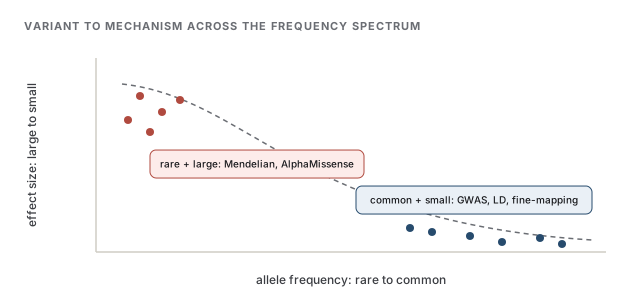
This shapes everything downstream. Genotyping arrays and most GWAS capture common variants, so they see a sea of tiny effects; catching the rare large-effect variants means sequencing many people. It also gives ML variant-effect predictors their training signal: models such as AlphaMissense lean on the fact that a variant common across humans and primates is probably tolerated, using frequency as a proxy for "benign" (Cheng et al., 2023). Population resources like gnomAD provide exactly these allele frequencies across ancestries, and nothing else: gnomAD carries no phenotypes, only who carries what and how often. Turning a flagged variant into a mechanism is the job of the variant-to-mechanism chapter (Chapter 13).

5.2GWAS, linkage, and heritability

A genome-wide association study (GWAS) is conceptually a giant loop: for each of millions of common SNPs, test whether carrying one allele versus the other correlates with a trait across a cohort. Because you run millions of tests, chance alone throws up small p-values, so the field uses a stringent genome-wide significance threshold of 5 times 10 to the minus 8, roughly a Bonferroni correction for the million-odd independent common variants in the genome.

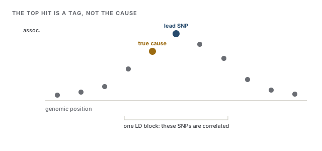
Now the trap. A significant SNP is almost never the variant that does the work. Variants close together on a chromosome are inherited as a block and are therefore correlated, a phenomenon called linkage disequilibrium (LD). When one variant in a haplotype block (a run of correlated variants) drives a trait, every variant correlated with it lights up too. The one with the smallest p-value, the lead SNP, is just the best-correlated tag for the causal signal, not necessarily the cause. A GWAS hit therefore localizes a region, typically tens to hundreds of variants wide, not a variant and certainly not a gene.

Heritability is the fraction of a trait's variation across people that is attributable to genetic differences, estimated classically from twins and families. SNP-heritability is the slice of that captured by common SNPs, estimated with methods that read the whole genome jointly rather than one hit at a time. For years there was a striking gap: the genome-wide-significant hits explained only a sliver of the heritability twins implied, the famous missing heritability. Much of it turned out to be hiding rather than truly missing, spread across thousands of sub-threshold variants each too weak to clear 5 times 10 to the minus 8 individually. This is polygenicity: most common traits are driven by a vast number of small effects. The omnigenic model pushes this further, arguing that because regulatory networks are densely interconnected, essentially every gene expressed in a relevant cell nudges the trait, so association signal is smeared across most of the genome rather than concentrated in an obvious pathway (Boyle et al., 2017).

5.3Association versus causation

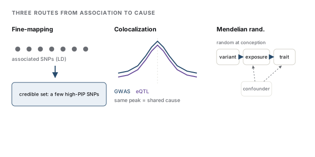
Getting from a region to a cause takes deliberate statistical work, and three tools do most of it.

Fine-mapping exploits the very LD structure that caused the problem. Given the correlations among variants in a region, methods like SuSiE (Sum of Single Effects) compute, for each variant, a posterior inclusion probability (PIP) that it is causal, and return a credible set: a small group of variants that together are highly likely to contain the true one (Wang et al., 2020). It narrows a hundred-variant tag into a handful, though it still cannot tell you which gene those variants act on.

Colocalization answers the gene question by borrowing molecular data. A QTL (quantitative trait locus) is a variant whose dose changes a molecular readout; an eQTL changes a gene's expression. Colocalization, implemented in tools like coloc, asks whether the GWAS signal and a nearby eQTL are driven by the same causal variant (Giambartolomei et al., 2014). When they colocalize, you have a candidate mechanism: this variant changes this gene's expression, which changes the trait. When they merely sit near each other by coincidence, you do not.

Mendelian randomization (MR) turns a variant into a natural experiment. Because alleles are shuffled randomly at conception, a variant that raises some exposure (LDL cholesterol, say) acts like an instrumental variable, a randomized nudge you can use to test whether the exposure causes an outcome rather than merely correlating with it. The analogy to a randomized trial is honest but leaks in one specific place: it holds only if the variant affects the outcome solely through that exposure. When a variant also acts through other pathways, called horizontal pleiotropy, the instrument is dirty and the causal estimate is biased, which is why careful MR studies test for and model this heterogeneity.

The final hazard is the one an ML practitioner will recognize instantly once named. Population stratification is confounding by ancestry: different ancestry groups differ in both allele frequencies and trait prevalence, so any allele that happens to be more common in one group tracks the trait for reasons that have nothing to do with biology. It is the exact genetic analogue of a batch effect (Chapter 4), and it is handled the same defensive way, by regressing out ancestry with genetic principal components or a mixed model before trusting any association. Miss it and your GWAS is measuring which population you sampled, not which variant matters.

References

- Boyle, E. A., Li, Y. I., & Pritchard, J. K. (2017). An Expanded View of Complex Traits: From Polygenic to Omnigenic. Cell.
- Cheng, J., Novati, G., Pan, J., Bycroft, C., Žemgulytė, A., Applebaum, T., Pritzel, A., Wong, L. H., et al. (2023). Accurate proteome-wide missense variant effect prediction with AlphaMissense. Science.
- Giambartolomei, C., Vukcevic, D., Schadt, E. E., Franke, L., Hingorani, A. D., Wallace, C., & Plagnol, V. (2014). Bayesian test for colocalisation between pairs of genetic association studies using summary statistics. PLoS Genetics.
- Wang, G., Sarkar, A., Carbonetto, P., & Stephens, M. (2020). A simple new approach to variable selection in regression, with application to genetic fine mapping. Journal of the Royal Statistical Society: Series B (Statistical Methodology).
Check yourself
Questions a sharp collaborator might ask on this chapter. Pick an answer to see whether it holds up.
-
Why do common genetic variants tend to have small individual effect sizes on traits?
The empty upper-right corner of the frequency-versus-effect plot is a selection phenomenon, not a measurement artifact. A large-effect deleterious allele lowers reproductive success and is removed before it can become common, so the common variants that survive are individually weak. This is also why ML predictors can treat high cross-species allele frequency as a proxy for benign. -
A GWAS lead SNP passes genome-wide significance. What is the most defensible conclusion?
Linkage disequilibrium makes every variant in a haplotype block rise together, so the smallest p-value marks the best tag, not necessarily the cause. Most GWAS hits are non-coding and act through regulation, and localizing the actual variant requires fine-mapping the correlated block rather than trusting the lead SNP. -
The bulk of the 'missing heritability' for common traits is now best explained by which account?
SNP-heritability estimates that read the whole genome jointly recover most of the gap, showing the signal was hiding in thousands of weak variants below the significance line rather than truly missing. This polygenic picture, taken to its extreme, is the omnigenic model: signal smeared across most of the genome. -
Colocalization analysis (as in coloc) is designed to test what?
Colocalization asks whether two signals at a locus share a causal variant, which is stronger than mere proximity. The tempting near-miss is the expression-trait correlation, which is closer to a TWAS-style test and can be confounded by two distinct nearby causal variants that coloc is specifically built to distinguish. -
Mendelian randomization treats a genetic variant as a natural experiment. Which assumption is most central to that being valid?
The instrumental-variable logic breaks under horizontal pleiotropy, when the variant reaches the outcome through routes other than the exposure. Random inheritance handles ordinary confounding, but a pleiotropic variant biases the causal estimate, which is why careful MR uses multiple instruments and tests for heterogeneity among their estimates. -
An ML practitioner will recognize population stratification most readily as which familiar problem?
Ancestry is a confounder that shifts allele frequencies and trait prevalence together, so an allele can track a trait purely because of where it was sampled. The fix mirrors batch-effect correction: regress out genetic principal components or use a mixed model before trusting any association.