3Modern ML and Foundation Models, Quickly

A foundation model turns a biological sequence into a vector of meaning, learned by chewing through mountains of unlabeled sequence, and that representation transfers to tasks it was never explicitly trained for. That single sentence is most of what you need to read the rest of this book. This chapter is a fast refresher on the machine learning you probably already half-know, retooled for biology: what a representation is, the three model families you will keep meeting, and why pretraining then transferring works. It assumes you can read a training loop and know what a gradient is, so we do not re-derive backpropagation. For the mechanics of transformers in full, see the companion volume, Foundations of Large Language Models; here we take just enough to build the mental model the biology chapters lean on.

3.1Representations and transformers

Start with the object every model consumes: a token, one discrete unit of the input. For a protein the natural token is an amino acid; for DNA it is a nucleotide, or a short k-mer or byte-pair chunk (a learned merge of frequent character runs, the same trick that tokenizes English). The first thing the model does is look each token up in a table and replace it with an embedding, a learned vector of a few hundred to a few thousand numbers. Training nudges those vectors so that biochemically or evolutionarily similar tokens land near each other, which is why an embedding space is more than a lookup: it is a geometry where distance means something.

A fixed embedding still gives every leucine the same vector no matter where it sits. Biology does not work that way; a residue's role depends on its neighbors and its long-range partners. Attention, the core operation of the transformer architecture (Vaswani et al., 2017), fixes this by letting each position read a weighted blend of every other position, so the vector for a residue becomes context-aware: the same amino acid in an active site and in a flexible loop end up with different representations. Stack many attention layers and the model builds representations that quietly encode structure, conservation, and function, without ever being told those words.

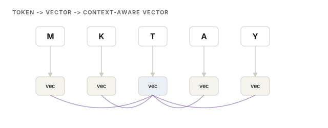
Why does this transfer? Because the pretraining task, predicting hidden or next tokens, is impossible to do well without internalizing the regularities that also govern the tasks you care about. A model that reliably guesses a masked residue has, along the way, learned which substitutions evolution tolerates, and that knowledge is exactly what a stability or variant-effect task needs.

3.2The model families you will meet

Almost every biology model in this book is one of three families, distinguished by how they factor probability and therefore by what they are good at.

Encoders (masked language models, in the style of BERT) see the whole sequence at once and are trained to fill in hidden tokens from both sides. Their output is a representation, one context-aware vector per token, so their job is understanding, not generation. This is the family behind protein models like ESM-2 (Lin et al., 2023) and ESM C, and DNA models like Nucleotide Transformer and DNABERT-2. Reach for an encoder when you want embeddings to feed a downstream predictor, or a per-site plausibility score.

Autoregressive decoders factor a sequence left to right, predicting each token from the ones before it. That factorization makes them natural generators: sample a token, feed it back, repeat. It also hands you a clean probability for any whole sequence, a measure of how "natural" it looks. Protein generators like ProGen2 and the genome model Evo 2 (Brixi et al., 2026), trained on 9.3 trillion nucleotides across the tree of life, live here. Reach for a decoder when you want to make new sequence or score whole-sequence likelihood.

Diffusion models learn to reverse a gradual noising process: start from noise and denoise, step by step, into a valid object. In biology that object is usually 3D coordinates, atoms of a protein backbone or a small molecule, where left-to-right generation makes no sense but iterative refinement does. AlphaFold3 pairs a transformer trunk with a diffusion head to predict all-atom structures of proteins with nucleic acids, ligands, and ions (Abramson et al., 2024), and RFdiffusion generates novel backbones for de novo design (Watson et al., 2023). Reach for diffusion when the answer is a shape.

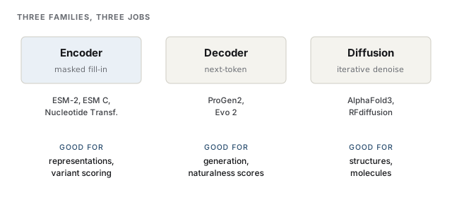
The boundaries blur in practice, and it helps to know where. ESM-3 is a generative masked model that reasons jointly over sequence, structure, and function, so it does not fit the tidy encoder box. AlphaFold3 is a transformer with a diffusion head. The families are a map of objectives, not a taxonomy of products.

3.3Pretraining, fine-tuning, zero-shot

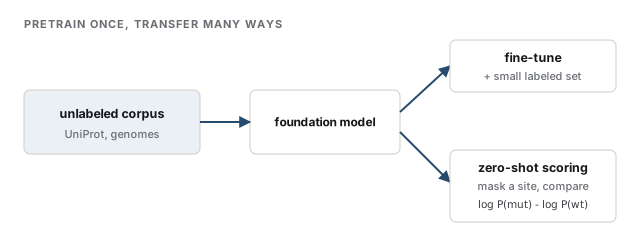
The reason these models exist at all is self-supervised pretraining: you train on a task whose labels come free from the data itself. Mask a residue and predict it; predict the next nucleotide. No experiment, no annotation, just raw sequence, which is the one thing biology has in abundance, in UniProt and metagenomic and genome databases. This is why a foundation model, a large model pretrained once on broad data, can then be pointed at many downstream tasks: the expensive learning already happened, off the labels you do not have.

You transfer that learning in three ways, in rough order of how much labeled data they need. Fine-tuning adds a small task head and continues training the weights on your labeled set (thousands of examples might do). A linear probe is the cheap cousin: freeze the model, fit a simple model on its frozen embeddings. And zero-shot prediction asks the pretrained model directly, with no task-specific training at all.

The zero-shot trick you will meet constantly is scoring a mutation by likelihood. To ask whether a variant is damaging, compare how probable the model finds the mutant residue versus the wild-type one at that site, the log-likelihood ratio log P(mutant) − log P(wild-type). A large negative number says the model, having learned what evolution permits, finds the mutation surprising, which correlates with functional damage. ESM-1v does exactly this and reaches roughly 0.5 Spearman correlation with deep mutational scans across dozens of proteins, matching older alignment-based methods with no per-protein training (Meier et al., 2021). Evo 2 runs the same play one level down, scoring genomic variants by their likelihood under a genome model.

References

- Abramson, J., Adler, J., Dunger, J., Evans, R., Green, T., Pritzel, A., Ronneberger, O., Willmore, L., et al. (2024). Accurate structure prediction of biomolecular interactions with AlphaFold 3. Nature.
- Brixi, G., Durrant, M. G., Ku, J., Naghipourfar, M., Poli, M., Sun, G., Brockman, G., Chang, D., et al. (2026). Genome modelling and design across all domains of life with Evo 2. Nature.
- Lin, Z., Akin, H., Rao, R., Hie, B., Zhu, Z., Lu, W., Smetanin, N., Verkuil, R., et al. (2023). Evolutionary-scale prediction of atomic-level protein structure with a language model. Science.
- Meier, J., Rao, R., Verkuil, R., Liu, J., Sercu, T., & Rives, A. (2021). Language models enable zero-shot prediction of the effects of mutations on protein function. NeurIPS.
- Vaswani, A., Shazeer, N., Parmar, N., Uszkoreit, J., Jones, L., Gomez, A. N., Kaiser, L., & Polosukhin, I. (2017). Attention Is All You Need. NeurIPS. arXiv:1706.03762.
- Watson, J. L., Juergens, D., Bennett, N. R., Trippe, B. L., Yim, J., Eisenach, H. E., Ahern, W., Borst, A. J., et al. (2023). De novo design of protein structure and function with RFdiffusion. Nature.
Check yourself
Questions a sharp collaborator might ask on this chapter. Pick an answer to see whether it holds up.
-
Why does self-supervised pretraining on unlabeled protein sequence transfer to a downstream task like stability prediction?
Transfer works because the pretraining objective is a hard proxy: a model that reliably fills in masked residues must have learned which substitutions evolution tolerates, and that knowledge overlaps with what stability tasks need. There are no stability labels or annotations in the raw sequence corpus, which is exactly why the free self-supervised signal is so valuable. -
You want to prioritize point mutations as likely damaging, with no labeled data for your protein. What do you compute?
Zero-shot variant scoring uses the log-likelihood ratio: a large negative value means the model finds the mutant surprising relative to wild-type, which correlates with damage. ESM-1v reaches about 0.5 Spearman with deep mutational scans this way, with no per-protein training. Embedding distance and attention weights are not calibrated to variant effect, and fine-tuning would defeat the point of a zero-shot method. -
A collaborator wants to generate a novel 3D protein backbone from scratch. Which model family is the natural fit, and why?
3D coordinates have no natural left-to-right order, so autoregressive generation is awkward; diffusion instead denoises a whole structure at once and is the basis of RFdiffusion and AlphaFold3's structure head. The family is fixed by the training objective, not by parameter count, which is why the same transformer blocks appear across all three families doing different jobs. -
A model assigns your engineered enzyme variant a high likelihood. Your collaborator concludes it will have higher catalytic activity. What is wrong with this reasoning?
Likelihood scores naturalness, a decent prior over plausible sequences, but your objective may pull away from what evolution produced; the two can diverge when you optimize for a designed goal. Evolution optimizes for organismal fitness under constraints, not for any single enzyme's turnover, so 'natural-looking' and 'best for my assay' are genuinely different targets. -
What most sharply distinguishes an autoregressive decoder like Evo 2 from a masked encoder like ESM-2?
The defining difference is the factorization: left-to-right for the decoder, which makes sampling natural, versus bidirectional masked fill-in for the encoder, which yields context-aware representations. Both are self-supervised and both can score sequences; encoders assign per-site pseudo-likelihoods even though they do not generate autoregressively, so 'encoders cannot score' is a common misconception.