2Deep Learning, Just Enough
Everything in this book runs on one engine: a differentiable function, a loss that scores its output, and gradient descent turning the loss into small parameter updates. You have seen all of this before. The job of this chapter is to compress it into the specific facts the later chapters lean on — how representations arise, what the training loop actually does, which optimizer LLMs use and why, why giant models generalize at all, and why the field settled on bf16. For the full course, the standard reference is still the Goodfellow, Bengio, and Courville textbook (Goodfellow et al., 2016); this is the refresher.
2.1From features to representations
Classical machine learning splits the work in two: a human designs features, and a model learns weights over them. Deep learning removes the split. You hand the network raw input — pixels, bytes, token ids — and each layer re-describes the output of the previous one, so the features themselves are learned. The early layers of a language model learn things like "these characters form a word"; later layers learn things like "this clause is the object of that verb." Nobody designed those features, and nobody could have designed the millions of stranger ones between them.
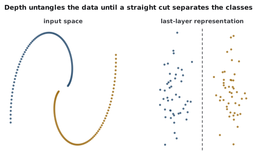
A useful geometric picture is the manifold view. Raw inputs are points tangled together in a huge space: sentences with opposite meanings can differ by one token. Each layer applies a learned transformation that untangles the manifold a little, so that by the final layer, things that should be treated the same sit near each other. Prediction becomes easy geometry at the top because the layers below did the unfolding.
Intuition
A deep network is not one clever function; it is a pipeline of small re-descriptions, each making the next layer's job slightly easier. "Depth" is how many times the input gets re-described.
2.2The training loop
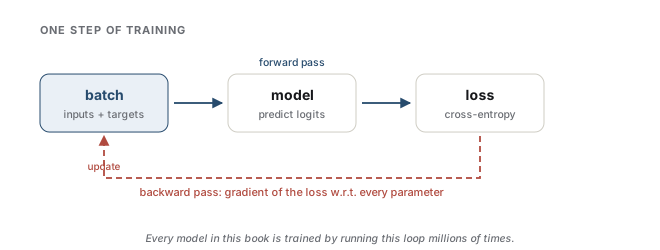
Every model in this book — from a toy MLP to a frontier LLM — is trained by the same five lines:
for batch in data:
    logits = model(batch.inputs)  # Forward pass.
    loss = cross_entropy(logits, batch.targets)  # How wrong were we?
    loss.backward()  # Backprop: compute every parameter's gradient.
    optimizer.step()  # Nudge every parameter downhill.
    optimizer.zero_grad()
The only non-obvious part is loss.backward(). Backpropagation (Rumelhart et al., 1986) is the chain rule from calculus, applied systematically from the loss backwards through every operation, reusing intermediate results so the whole thing costs about as much as the forward pass. Autograd frameworks are bookkeeping for that chain rule — they record what the forward pass did, then replay it in reverse. There is nothing else in the box: when Chapter 7 talks about a trillion-token pretraining run, it is this loop, run a few million times on a few thousand GPUs.
Analogy
Backprop is blame assignment on an assembly line. A defect is found at final inspection (the loss), and a memo travels backwards station by station, telling each worker how much their step contributed and in which direction to adjust. The analogy leaks in one way: on a real assembly line workers adjust one at a time, while gradient descent adjusts every station simultaneously — which is why each step must be small, or the workers invalidate each other's corrections.
2.3Optimizers and learning rates
Plain stochastic gradient descent takes the gradient of the current batch and steps against it. Two refinements matter, and they are the two knobs worth understanding:
- Momentum keeps a running average of recent gradients and steps along that instead. Individual batches are noisy; the average points where the loss is consistently going down.
- Adaptive scaling gives each parameter its own effective step size, normalized by the recent magnitude of its gradients. A parameter whose gradients are habitually huge takes proportionally smaller steps, and vice versa.
Adam (Kingma & Ba, 2015) combines both, and AdamW (Loshchilov & Hutter, 2019) fixes a subtle interaction with weight decay. The subtlety: if you add decay as an L2 penalty in the loss, it enters the gradient and is then divided by Adam's per-parameter denominator, so parameters with large gradients get less effective decay — the opposite of uniform. AdamW decouples the two, subtracting a fixed fraction of each weight directly, independent of gradient scale. AdamW is the default optimizer for essentially every LLM you will meet in this book, and Chapter 7 covers the learning-rate schedule (warmup, then decay) that accompanies it.
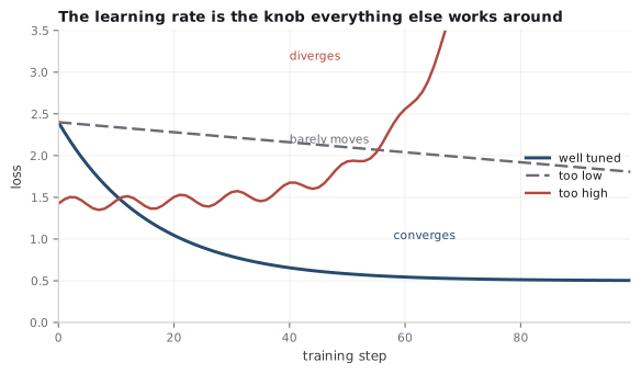
The learning rate itself remains the single most important hyperparameter in deep learning. Too high and the loss diverges; too low and you waste compute crawling. Everything else in an optimizer exists to make one global learning rate workable across millions of very different parameters.
Interview
Why is Adam(W) used for transformers instead of plain SGD? Because gradient magnitudes in a transformer vary enormously across parameters — embedding rows for rare tokens see gradients rarely, while LayerNorm gains see them constantly. Adam's per-parameter normalization equalizes these scales so one learning rate serves all of them; with plain SGD, transformers train poorly or need impractical per-layer tuning.
Interview
A model runs a forward pass fine but hits out-of-memory during training. Why, and what are your levers? Training holds far more than the weights: every layer's activations (kept for the backward pass), the gradients, and the optimizer state — for AdamW that is two moments per parameter plus, in mixed-precision training, an fp32 master copy, roughly 16 bytes per parameter before activations. The levers each attack one term: gradient checkpointing recomputes activations instead of storing them, gradient accumulation shrinks the batch's activation footprint, and optimizer-state sharding across GPUs (ZeRO, Chapter 8) splits the moments and master weights. Inference needs none of this, which is why a model that generates comfortably can still be untrainable on the same hardware.
2.4Regularization and generalization
The classical story says a model with too many parameters will memorize its training set and fail on new data, so you constrain it: weight decay shrinks weights toward zero, and dropout (Srivastava et al., 2014) randomly silences activations during training so no unit can depend too much on another.
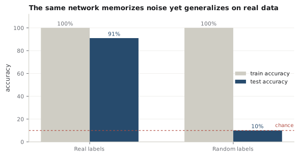
LLMs complicate the classical story twice. First, the puzzle: modern networks are so overparameterized that they can memorize completely random labels — yet the same architectures, trained on real data, generalize well (Zhang et al., 2017). Capacity alone does not decide generalization; what the optimizer finds first, and the structure in the data, matter more than the parameter count. Second, the practice: a pretraining run makes roughly one pass over its enormous corpus, so the model rarely sees any example twice — classic overfitting has little room to happen. Weight decay survives in LLM training more as a stabilizer than as an anti-memorization device, and dropout has largely disappeared from pretraining.
Intuition
Overfitting is a symptom of revisiting the same data with too much capacity. Pretraining starves it from the data side: with trillions of tokens seen once, the model has no choice but to learn patterns, because memorization has nothing to grab onto twice.
2.5Numerical precision
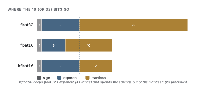
A number format spends its bits on two things: dynamic range (how large and small the exponent lets values get) and precision (how many mantissa bits distinguish nearby values). float32 has plenty of both but costs 4 bytes per number — memory and bandwidth you will learn to resent in Parts II and IV.
The two half-size formats split the budget differently:
| Format | Exponent bits | Mantissa bits | Range | Precision |
|---|---|---|---|---|
| float32 | 8 | 23 | huge | high |
| float16 | 5 | 10 | narrow | medium |
| bfloat16 | 8 | 7 | same as float32 | low |
fp16's narrow range is the problem: gradients in a large model span many orders of magnitude, and values silently underflow to zero or overflow to infinity. Training in fp16 requires loss scaling — multiplying the loss so gradients sit inside the representable window — and it is fragile machinery (Micikevicius et al., 2018). bf16 keeps float32's full exponent, sacrificing precision instead (Kalamkar et al., 2019). That trade wins because training is noisy anyway: stochastic gradients already jitter far more than the mantissa error, but a single overflow can kill a run.
Interview
Why did bf16 beat fp16 for training? Because training tolerates noise but not clipped range. bf16 keeps float32's 8-bit exponent, so nothing overflows or underflows and no loss scaling is needed; the precision it gives up disappears into gradient noise the run already has. fp16 spends its bits the other way and buys a failure mode instead.
Precision returns in Chapter 16 from the other side: at inference time, weights are static and the noise argument changes, which is why quantization can push below 8 bits per weight when training cannot.
That is the equipment. Next, the specific way LLMs turn text into the integers this machinery consumes.
References
- Goodfellow, I., Bengio, Y., & Courville, A. (2016). Deep learning. MIT Press.
- Kalamkar, D., Mudigere, D., Mellempudi, N., Das, D., et al. (2019). A study of BFLOAT16 for deep learning training. arXiv preprint. arXiv:1905.12322.
- Kingma, D. P., & Ba, J. (2015). Adam: A method for stochastic optimization. International Conference on Learning Representations. arXiv:1412.6980.
- Loshchilov, I., & Hutter, F. (2019). Decoupled weight decay regularization. International Conference on Learning Representations. arXiv:1711.05101.
- Micikevicius, P., Narang, S., Alben, J., Diamos, G., et al. (2018). Mixed precision training. International Conference on Learning Representations. arXiv:1710.03740.
- Rumelhart, D. E., Hinton, G. E., & Williams, R. J. (1986). Learning representations by back-propagating errors. Nature, 323.
- Srivastava, N., Hinton, G., Krizhevsky, A., Sutskever, I., & Salakhutdinov, R. (2014). Dropout: A simple way to prevent neural networks from overfitting. Journal of Machine Learning Research, 15(56).
- Zhang, C., Bengio, S., Hardt, M., Recht, B., & Vinyals, O. (2017). Understanding deep learning requires rethinking generalization. International Conference on Learning Representations. arXiv:1611.03530.
Check yourself
Interview-style questions on this chapter. Pick an answer to see whether it holds up.
-
Your model runs a forward pass on a batch just fine, but the same batch runs out of memory during training. What is the primary reason, and which lever most directly addresses it?
Inference needs only the weights and a single layer's activations. Training additionally holds every layer's activations (for the backward pass), the gradients, and the optimizer state; for AdamW that is two moments plus commonly an fp32 master copy, roughly 16 bytes per parameter before activations. Gradient checkpointing recomputes activations in the backward pass instead of storing them; sharding (ZeRO, Chapter 8) and gradient accumulation are the other levers. -
What is the actual difference between L2 regularization folded into the loss and AdamW's decoupled weight decay?
Adam normalizes each parameter's update by a running estimate of its gradient magnitude. If weight decay rides in through the gradient (L2 in the loss), it gets rescaled by that same denominator and becomes uneven across parameters. AdamW decouples the two, subtracting a fixed fraction of each weight directly, which is why it is the default for transformers. -
The same overparameterized network can be trained to 100% accuracy on data with completely random labels, yet it generalizes well on real labels. What does this most directly imply?
Zhang et al. (2017) showed capacity is enough to memorize noise, so classical bounds tying capacity to generalization cannot be the whole story. On structured data the optimizer tends to find simpler, better-generalizing solutions first. In pretraining, a near-single pass over a huge corpus also removes most of the opportunity to memorize. -
Why did bfloat16 become the default over float16 for training, even though float16 offers more mantissa bits (higher precision)?
Training tolerates noise but not clipped range. float16's narrow 5-bit exponent forces fragile loss-scaling to keep gradients representable; bfloat16 spends its bits on range instead of precision, so nothing silently flushes to zero or infinity. Both are 16 bits, so memory is the same. -
Why is Adam(W) preferred over plain SGD for transformers specifically?
A transformer mixes parameters whose gradients differ by orders of magnitude and by how often they are exercised. Adam gives each parameter an effective step size scaled by its own recent gradient magnitude, so one learning rate serves all of them; plain SGD would need impractical per-layer tuning.