16Quantization
A trained model is a pile of numbers, and by default each one is a 16-bit float. Quantization asks a blunt question: do you really need 16 bits per weight, or would 8, or 4, do almost as well? The answer, for inference, is usually "far fewer than you think." Dropping from 16-bit to 4-bit shrinks a model roughly four times and — because generating a token is bottlenecked on reading weights out of memory, not on arithmetic (Appendix A) — makes it about four times faster, for a quality cost that is often close to noise. This chapter is about how that trade is made, where it breaks, and which of the confusing zoo of formats you will actually reach for.
16.1Bits, ranges, and where the memory goes
At inference the weights dominate memory. A dense model reads every weight once per generated token, so the model's footprint is close to parameters × bytes-per-weight, and the KV cache (Chapter 15) rides on top. That single product is the whole reason quantization exists: halve the bytes per weight and you halve both the memory the model occupies and the bytes you must stream to produce each token. Training is a different story — there the optimizer state, not the weights, is the giant (Chapter 8) — but for a frozen model being served, the weights are the bill.
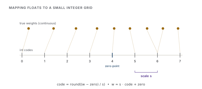
So the goal is fewer bits per weight without wrecking the model. Quantization does it by mapping each weight from a continuous float to one rung of a small, evenly spaced integer ladder. You pick a scale \(s\) (the spacing between rungs) and an optional zero-point \(z\) (which integer stands in for the value zero), then store the integer code and reconstruct the weight on demand:
With \(b\) bits you get \(2^b\) rungs, so 4-bit quantization approximates every weight in a tensor with just sixteen distinct values. The art is choosing \(s\) and \(z\) so the ladder covers the weights that matter without wasting rungs on empty range.
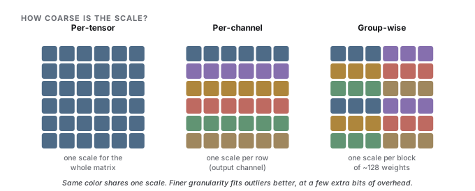
The catch is that one scale has to serve many weights, and a single outlier stretches the ladder so far that ordinary weights collapse onto a handful of rungs. The fix is granularity: share a scale over a smaller region. Per-tensor uses one scale for the whole matrix (cheapest, crudest); per-channel gives each output row its own scale; group-wise goes finer still, one scale per contiguous block of typically 64 or 128 weights. Finer granularity tracks local variation better and costs only the handful of extra bytes those extra scales take — which is why essentially every modern 4-bit scheme is group-wise.
Intuition
A weight matrix is a photograph and quantization is saving it with fewer colors. One palette for the whole image (per-tensor) blows the budget on a lone bright pixel; a fresh palette per small tile (group-wise) keeps detail everywhere for a negligible bookkeeping cost.
16.2Post-training quantization
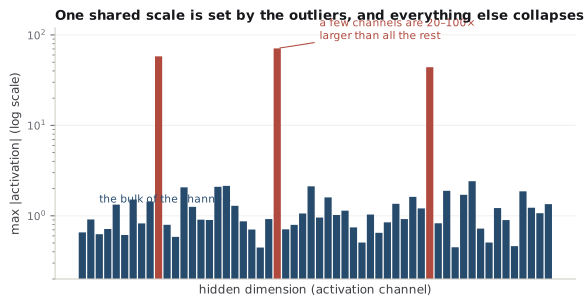
The cheapest path is post-training quantization (PTQ): take a finished model and quantize it directly, no gradient descent required. The naive version — round every weight to its nearest rung — works passably down to 8 bits and falls apart at 4, and the reason is outliers. In a trained transformer, a few activation dimensions carry magnitudes tens to hundreds of times larger than the rest, and these emergent "outlier features" appear in essentially every large model past a few billion parameters (Dettmers et al., 2022). A scale wide enough to represent them leaves every ordinary value crushed into a few rungs.
Two families answer the spikes. The first is weight-only quantization, which keeps activations in 16-bit and only compresses the weights — the common case, since weights are the memory and bandwidth bill. GPTQ quantizes weights one column at a time and uses second-order (Hessian) information from a small calibration set to adjust the not-yet-quantized weights so they compensate for the rounding error just introduced, holding accuracy near 4 bits (Frantar et al., 2023). AWQ starts from a sharper observation: not all weights matter equally, and the salient ones are identifiable from the activation magnitudes they multiply. It protects that roughly 1% by scaling those channels up before quantizing (and back down after), so the important weights land on the ladder with less error (Lin et al., 2024). Both lean on calibration data — a few hundred representative sequences run through the model to measure the activation statistics that set the scales. It is a light touch, not training, but it is why a domain-matched calibration set beats a random one.
The second family is weight-and-activation quantization, which pushes activations down to 8-bit integers too so the matrix multiplies themselves run in INT8 — a real compute win, not just a memory one. That runs straight into the outliers, and here the clever move is to move the difficulty rather than fight it. SmoothQuant observes that weights are easy to quantize and activations are hard, so it migrates the pain: it divides each outlier activation channel by a per-channel constant and multiplies the corresponding weight column by the same constant, an exactly equivalent rewrite that leaves the math unchanged while flattening the activations into a quantizable range (Xiao et al., 2023). The predecessor, LLM.int8(), took a blunter route: run the 99.9% of well-behaved dimensions in INT8 and peel the few outlier dimensions off into a 16-bit side computation, a mixed-precision decomposition that preserves quality at the cost of a more complex kernel (Dettmers et al., 2022).
Interview
Why does naive 4-bit quantization destroy an LLM when it barely dents a ResNet? Emergent activation outliers. Large language models develop a few feature dimensions with enormous magnitude, and a scale stretched to cover them collapses everything else. The fixes either isolate the outliers (LLM.int8()), migrate their difficulty into the weights (SmoothQuant), or protect the salient weights the outliers multiply (AWQ). A vision CNN has no comparable outlier structure, so per-tensor rounding just works.
Common trap
"Weight-only 4-bit" and "W4A8" are not the same claim. Weight-only shrinks memory and decode bandwidth but still computes in 16-bit, so it does nothing for a compute-bound prefill on a long prompt. Quantizing activations too is what unlocks integer matmuls — and what forces you to confront outliers head-on. Know which one a "4-bit" number refers to before you quote its speedup.
16.3Formats you'll meet: GGUF, bitsandbytes, MLX
The research above ships to you as a few concrete formats, and knowing which is for what saves a lot of confusion. They differ less in the underlying idea than in the runtime they target.
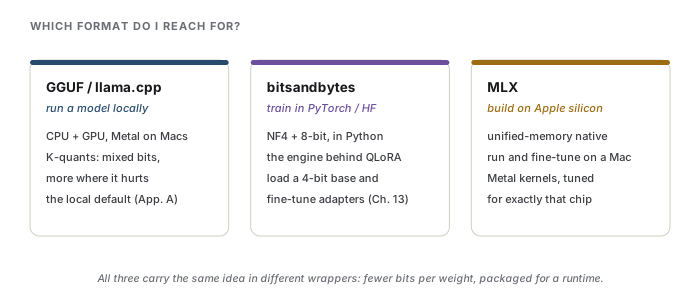
GGUF is the model container used by llama.cpp, the C/C++ engine most local inference runs on (Appendix A). Its signature is the family of K-quants — schemes named like Q4_K_M that mix precision within a model, spending more bits on the layers and tensors that are most sensitive (attention and the parts that hurt most when degraded) and fewer on the rest. That mixing is why a 4-bit GGUF build holds up better than a flat 4-bit round: the bit budget goes where it earns its keep. Q4_K_M is the usual quality-versus-size sweet spot people download.
bitsandbytes is the quantization layer inside the PyTorch and Hugging Face stack. It gives you 8-bit and 4-bit tensors you can drop into a model in Python, and it is the engine under QLoRA: its NF4 (NormalFloat4) type is a 4-bit format whose rungs are spaced to match the roughly-Gaussian distribution of neural-network weights, so the ladder puts more rungs where the weights actually cluster (Chapter 13) (Dettmers et al., 2023). Reach for it when you want to load and train against quantized weights, not just run them.
MLX is Apple's array framework, built for Apple-silicon unified memory. It carries its own quantized types and Metal kernels and is the path when you want to run or fine-tune on a Mac and get the best out of that specific hardware. The practical decision is short: GGUF/llama.cpp to run a model locally, bitsandbytes to train one in PyTorch, MLX when you are on a Mac and want the native path — a picture Appendix A works through end to end.
Interview
A teammate says "just use Q4." What do you ask? First, which task and hardware: Q4_K_M is a great default for local chat on llama.cpp, but a throughput server running vLLM or TensorRT-LLM wants a GPTQ or AWQ build with INT8/INT4 kernels, not GGUF. Second, weight-only or weights-plus-activations, since only the latter speeds up prefill. Third, was it calibrated on data resembling the target domain? "Q4" names a size, not a method or a quality.
16.4Quantization-aware training and the frontier
PTQ treats quantization as something done to a finished model. Quantization-aware training (QAT) instead lets the model learn to be good at low precision: during training you insert "fake quantization" that rounds weights and activations on the forward pass while letting gradients flow through the rounding (a straight-through estimator), so the model adapts its weights to the coarse ladder it will be served on. QAT costs a training run but pays off exactly where PTQ starts to hurt — at very low bit-widths — because the model can arrange its weights to survive rounding rather than being rounded after the fact. Recent open models ship a QAT variant for this reason.
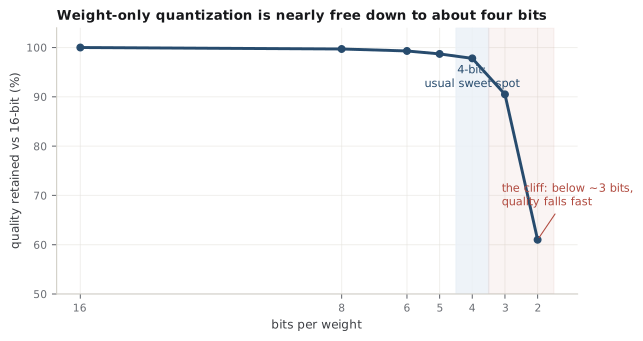
Where does it start to hurt? Weight-only quantization is nearly free down to about 4 bits, and then quality falls off a cliff. The gap from 16-bit is a rounding error at 8 bits, still small at 4, and then 3-bit and 2-bit PTQ degrade sharply — the model runs out of rungs to represent the distinctions it needs. QAT and better group-wise schemes push the cliff edge lower, but they do not abolish it.
Intuition
PTQ asks a trained model to tolerate a coarser ruler after the fact; QAT lets the model learn while holding that coarser ruler. The second always tolerates a shorter ruler, because the model gets to arrange itself around the marks it will actually have.
The frontier in 2026 has moved the low-precision idea into training itself. Where quantization was long an inference-only afterthought, DeepSeek-V3 trained a 671B model natively in FP8 — 8-bit floats, with fine-grained block-wise scaling and a few sensitive components kept in higher precision — cutting training compute and memory without losing accuracy (DeepSeek-AI, 2024). The next step down is already shipping: FP4 microscaling formats (MXFP4 and NVFP4, 4-bit floats with a shared block scale, accelerated on current hardware) now back both inference and, increasingly, training. OpenAI's open gpt-oss models were released with their mixture-of-experts weights — about 90% of the parameters — stored natively in MXFP4, so the released checkpoint is the 4-bit model rather than a lossy compression of a 16-bit one. The throughline of the whole chapter: the field keeps discovering that models need far fewer bits than anyone assumed, and the only durable question is where on the bits-versus-quality curve a given deployment should sit.
Interview
Is QLoRA quantization-aware training? No, and the distinction is a favorite probe. QLoRA stores a frozen base in 4-bit NF4 only to save memory, dequantizing each weight to 16-bit for its matmul while the learning happens in separate 16-bit LoRA adapters (Chapter 13); the base is never trained at 4-bit. QAT trains the model to be good at low-precision inference. One is a memory trick for fine-tuning; the other is how you make a genuinely 4-bit model that stays accurate.
The next chapter turns from making the weights small to making the whole serving stack fast: batching, paging the KV cache, and the engines that tie quantization, attention, and scheduling into a system that serves thousands of users at once.
References
- DeepSeek-AI (2024). DeepSeek-V3 technical report. arXiv preprint. arXiv:2412.19437.
- Dettmers, T., Lewis, M., Belkada, Y., & Zettlemoyer, L. (2022). LLM.int8(): 8-bit matrix multiplication for transformers at scale. Advances in Neural Information Processing Systems. arXiv:2208.07339.
- Dettmers, T., Pagnoni, A., Holtzman, A., & Zettlemoyer, L. (2023). QLoRA: Efficient finetuning of quantized LLMs. Advances in Neural Information Processing Systems. arXiv:2305.14314.
- Frantar, E., Ashkboos, S., Hoefler, T., & Alistarh, D. (2023). GPTQ: Accurate post-training quantization for generative pre-trained transformers. International Conference on Learning Representations. arXiv:2210.17323.
- Lin, J., Tang, J., Tang, H., Yang, S., et al. (2024). AWQ: Activation-aware weight quantization for LLM compression and acceleration. Proceedings of Machine Learning and Systems (MLSys). arXiv:2306.00978.
- Xiao, G., Lin, J., Seznec, M., Wu, H., Demouth, J., & Han, S. (2023). SmoothQuant: Accurate and efficient post-training quantization for large language models. International Conference on Machine Learning. arXiv:2211.10438.
Check yourself
Interview-style questions on this chapter. Pick an answer to see whether it holds up.
-
Naive round-to-nearest quantization takes a large language model to 4 bits and its outputs turn to garbage, yet the same recipe barely dents a vision CNN of similar size. What is the root cause specific to the LLM?
The culprit is emergent activation outliers (Dettmers et al., 2022): past a few billion parameters, a small set of feature dimensions blow up in magnitude, and a per-tensor scale stretched to represent them leaves everything else with almost no resolution. The heavy-tailed weights option is the tempting near-miss — weight shape does motivate formats like NF4 — but it is not what breaks naive 4-bit; the activation outliers are, which is why LLM.int8(), SmoothQuant, and AWQ all target them. -
SmoothQuant and AWQ both fight activation outliers, but their mechanisms differ. Which pair of descriptions is correct?
SmoothQuant (Xiao et al., 2023) applies a per-channel constant that divides the hard-to-quantize activations and multiplies the corresponding weight columns, an exactly equivalent rewrite that moves the difficulty to the easy-to-quantize weights. AWQ (Lin et al., 2024) identifies salient weights from activation statistics and scales them to reduce their rounding error. The tempting scramble mixes up the method names: the keep-outliers-in-16-bit trick is LLM.int8() and the Hessian correction is GPTQ, neither of which is SmoothQuant or AWQ. -
You quantize a 13B model weight-only to 4 bits and measure a large speedup on decoding long responses, but almost none on processing long prompts. Why?
Weight-only 4-bit stores weights in 4 bits but dequantizes them to 16-bit for the actual matmul, so it buys memory and decode bandwidth, not arithmetic. Prefill is compute-bound and parallel, so it sees little benefit; decode streams every weight from memory per token, so halving the bytes roughly halves the time. To speed prefill you must quantize activations too (W8A8) and run genuine integer matmuls — a different, harder regime because of outliers. -
In a GGUF 'Q4_K_M' build for llama.cpp, what does the K-quant scheme actually do, and why does it beat rounding every weight to a flat 4 bits?
K-quants use mixed precision across tensors — more bits for the sensitive parts (such as attention projections), fewer elsewhere — so the same average bit-width preserves more quality than a uniform round. The Gaussian-spaced-rungs option describes NF4 (bitsandbytes/QLoRA), a real but different idea, which makes it the tempting near-miss; and K-quants are post-training, not QAT, and remain weight-only rather than quantizing activations. -
An interviewer asks whether QLoRA is a form of quantization-aware training. What is the accurate answer?
QLoRA (Dettmers et al., 2023) keeps 4-bit NF4 purely to fit the frozen base in memory; every weight is dequantized to 16-bit for its multiply, and all learning lives in 16-bit LoRA adapters that are themselves not quantized. QAT, by contrast, trains the model to be accurate at low-precision inference via fake quantization on the forward pass. The trap is the claim that the LoRA adapters are themselves fake-quantized 4-bit tensors: they are trained in full precision, not at 4 bits.