5How Modern Architectures Differ

Chapter 4 built the transformer as published in 2017 (Vaswani et al., 2017). No frontier model ships that exact recipe anymore — and yet the changes are few, and every one of them fixes a specific pain: training instability, KV-cache memory, or compute per token. This chapter walks the modern substitutions one component at a time. By the end you can read a real model's config file line by line, which is exactly how the chapter closes. The recipe below (rotary positions, pre-norm RMSNorm, SwiGLU, grouped-query attention) crystallized in the Llama family (Touvron et al., 2023) and is now close to universal for open models.

5.1Positional information: RoPE

Attention is order-blind: shuffle the tokens and the \(QK^\top\) scores shuffle with them. The original transformer injected order by adding a position vector to each token embedding at the bottom of the stack. That works, but position becomes just another ingredient blended into the residual stream, and attention only sees it indirectly.

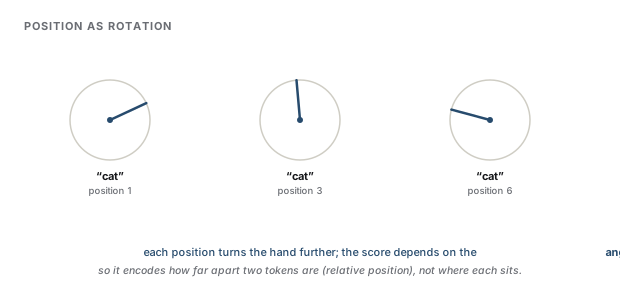
Rotary position embeddings (RoPE) (Su et al., 2024) move position into the attention scores themselves. Split each query and key vector into two-dimensional pairs, and rotate each pair by an angle proportional to the token's position, with each pair rotating at its own frequency. The payoff is in the dot product: the score between a query at position \(m\) and a key at position \(n\) depends only on the offset \(m-n\), not on the absolute positions. Relative position falls out of the geometry.

RoPE also concentrates the levers for long context: because position lives in rotation frequencies, stretching the frequency schedule is how a model trained at one context length is extended to a much longer one. The named methods — linear position interpolation, NTK-aware scaling, and YaRN (Peng et al., 2023) — differ in how carefully they remap those frequencies so that short-range resolution survives; the serving costs return in Chapter 15.

5.2Normalization: RMSNorm and pre-norm

Two separate upgrades hide under "normalization."

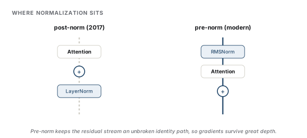
Where it sits: the 2017 transformer normalized after each sublayer (post-norm), which at large depth needs a delicate warmup to avoid divergence. Placing the normalization before each sublayer (pre-norm) keeps the residual stream itself untouched — an identity path from embedding to output — and gradients flow through deep stacks without drama (Xiong et al., 2020). Every modern LLM is pre-norm; the block in Chapter 4 already showed it.

What it computes: LayerNorm (Ba et al., 2016) centers activations (subtract the mean) and scales them (divide by the standard deviation). RMSNorm (Zhang & Sennrich, 2019) drops the centering and simply divides by the root-mean-square, with a learned gain. It is cheaper — one fewer reduction over the hidden dimension, and no bias parameters — and models train just as well. When an ablation says the cheap half of an operation was the only half that mattered, the expensive half disappears from the recipe.

A related trick you will see in recent models is QK-norm: normalizing the queries and keys before their dot product to keep attention logits from blowing up at large scale (Dehghani et al., 2023).

5.3Activations: SwiGLU

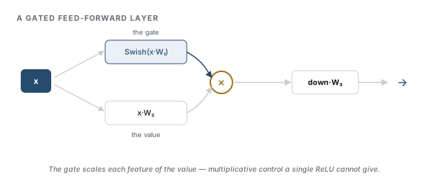
The original FFN is two matrices with a ReLU between them. Modern models use a gated unit instead: project the input up twice, let one projection gate the other elementwise, then project back down,

The gate lets the layer modulate how much of each feature passes, not just whether it is positive — multiplicative control instead of a hard one-sided switch. Across GLU variants, SwiGLU reliably wins by a small margin (Shazeer, 2020).

There is one bookkeeping consequence you will see in every config: SwiGLU has three matrices where the classic FFN has two, so to hold the parameter count fixed, the hidden width shrinks from \(4d\) to roughly \(\tfrac{2}{3} \cdot 4d\). That is why real models have oddly specific FFN sizes instead of a clean \(4d\).

5.4Attention variants: MQA and GQA

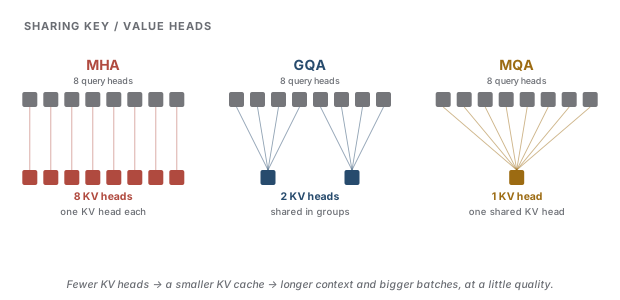
At inference time, every past token's keys and values are cached so they are not recomputed per step — the KV cache, whose memory math Chapter 15 and Appendix A work out. In full multi-head attention, every head stores its own keys and values, so the cache scales with the head count, and at long context it competes with the weights for memory and bandwidth.

The fix is to share. Multi-query attention (MQA) keeps all the query heads but gives them one shared key/value head (Shazeer, 2019) — a large cache reduction with a measurable quality cost. Grouped-query attention (GQA) interpolates: query heads are divided into groups, each group sharing one KV head (Ainslie et al., 2023). With, say, 32 query heads and 8 KV heads, the cache shrinks 4× while quality stays near full multi-head attention. GQA is the current default.

Sharing heads is not the only lever on the cache. Sliding-window (local) attention bounds it a different way: each token attends only to the last \(w\) tokens, so cost and cache stop growing once the window is full, often with a few global layers interleaved to preserve long-range reach (Jiang et al., 2023). And multi-head latent attention (MLA), the successor probe past GQA, compresses the keys and values into a small shared latent, shrinking the cache below what GQA achieves (DeepSeek-AI, 2024).

5.5Mixture of experts

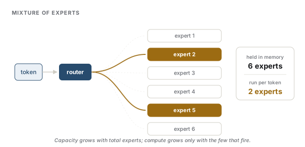
Everything so far tweaks the dense recipe. Mixture of experts (MoE) changes the deal: replace each FFN with many parallel FFNs (experts) plus a small router that sends each token to its top one or two experts (Shazeer et al., 2017; Fedus et al., 2022). The model's total parameters multiply, but the compute per token only touches the chosen experts.

That splits a number you have been treating as one. A "Mixtral 8×7B" has ~47B total parameters (what you must hold in memory) but only ~13B active parameters per token (what you pay compute and, per Appendix A, bandwidth for). Scaling laws (Chapter 9) say capacity buys quality; MoE buys capacity without buying per-token compute.

The costs are real, and the routing details are where the interviews live. Each expert has a capacity; tokens routed past it are dropped, so the router must be trained to spread load evenly. Classic MoE adds an auxiliary load-balancing loss for this; because that loss tugs against quality, newer models (DeepSeek-V3) pursue auxiliary-loss-free balancing via learned routing biases instead (DeepSeek-AI, 2024). All experts must also fit in memory even though most idle per token, training is less stable than dense, and Chapter 8's parallelism grows a new dimension since experts can live on different devices.

5.6A tour of a current open model

Here is the config of a Llama-3-class 8B model (Grattafiori et al., 2024), trimmed to the load-bearing fields:

{
  "hidden_size": 4096,
  "num_hidden_layers": 32,
  "num_attention_heads": 32,
  "num_key_value_heads": 8,
  "intermediate_size": 14336,
  "hidden_act": "silu",
  "rms_norm_eps": 1e-05,
  "rope_theta": 500000.0,
  "max_position_embeddings": 8192,
  "vocab_size": 128256
}

Read it with this chapter in hand. num_key_value_heads: 8 against 32 attention heads is GQA with groups of four — a 4× smaller KV cache. intermediate_size: 14336 is \(3.5d\), not \(4d\): the SwiGLU two-thirds bookkeeping, rounded to hardware-friendly multiples, with hidden_act: silu naming the Swish gate. rms_norm_eps tells you normalization is RMSNorm, and rope_theta: 500000 is the rotation base — raised well above the original \(10{,}000\) for longer context. The vocabulary of 128k tokens is Chapter 3's tradeoff, sized generously to shorten sequences. Every line is one of this chapter's sections, frozen into JSON.

The architecture is now current.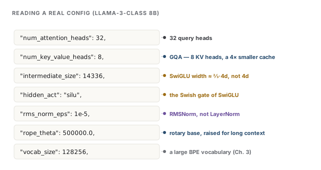

The next part of the book takes these frozen blueprints and asks how the weights inside them are actually learned.

References

- Ainslie, J., Lee-Thorp, J., de Jong, M., Zemlyanskiy, Y., Lebrón, F., & Sanghai, S. (2023). GQA: Training generalized multi-query transformer models from multi-head checkpoints. Empirical Methods in Natural Language Processing. arXiv:2305.13245.
- Ba, J. L., Kiros, J. R., & Hinton, G. E. (2016). Layer normalization. arXiv preprint. arXiv:1607.06450.
- DeepSeek-AI (2024). DeepSeek-V2: A strong, economical, and efficient mixture-of-experts language model. arXiv preprint. arXiv:2405.04434.
- DeepSeek-AI (2024). DeepSeek-V3 technical report. arXiv preprint. arXiv:2412.19437.
- Dehghani, M., Djolonga, J., Mustafa, B., Padlewski, P., et al. (2023). Scaling vision transformers to 22 billion parameters. International Conference on Machine Learning. arXiv:2302.05442.
- Fedus, W., Zoph, B., & Shazeer, N. (2022). Switch transformers: Scaling to trillion parameter models with simple and efficient sparsity. Journal of Machine Learning Research, 23(120). arXiv:2101.03961.
- Grattafiori, A., Dubey, A., Jauhri, A., Pandey, A., et al. (2024). The Llama 3 herd of models. arXiv preprint. arXiv:2407.21783.
- Jiang, A. Q., Sablayrolles, A., Mensch, A., Bamford, C., et al. (2023). Mistral 7B. arXiv preprint. arXiv:2310.06825.
- Peng, B., Quesnelle, J., Fan, H., & Shippole, E. (2023). YaRN: Efficient context window extension of large language models. International Conference on Learning Representations. arXiv:2309.00071.
- Shazeer, N., Mirhoseini, A., Maziarz, K., Davis, A., Le, Q., Hinton, G., & Dean, J. (2017). Outrageously large neural networks: The sparsely-gated mixture-of-experts layer. International Conference on Learning Representations. arXiv:1701.06538.
- Shazeer, N. (2019). Fast transformer decoding: One write-head is all you need. arXiv preprint. arXiv:1911.02150.
- Shazeer, N. (2020). GLU variants improve transformer. arXiv preprint. arXiv:2002.05202.
- Su, J., Ahmed, M., Lu, Y., Pan, S., Bo, W., & Liu, Y. (2024). RoFormer: Enhanced transformer with rotary position embedding. Neurocomputing, 568. arXiv:2104.09864.
- Touvron, H., Lavril, T., Izacard, G., Martinet, X., et al. (2023). LLaMA: Open and efficient foundation language models. arXiv preprint. arXiv:2302.13971.
- Vaswani, A., Shazeer, N., Parmar, N., Uszkoreit, J., Jones, L., Gomez, A. N., Kaiser, Ł., & Polosukhin, I. (2017). Attention is all you need. Advances in Neural Information Processing Systems. arXiv:1706.03762.
- Xiong, R., Yang, Y., He, D., Zheng, K., Zheng, S., Xing, C., Zhang, H., Lan, Y., Wang, L., & Liu, T.-Y. (2020). On layer normalization in the transformer architecture. International Conference on Machine Learning. arXiv:2002.04745.
- Zhang, B., & Sennrich, R. (2019). Root mean square layer normalization. Advances in Neural Information Processing Systems. arXiv:1910.07467.
Check yourself
Interview-style questions on this chapter. Pick an answer to see whether it holds up.
-
Rotary position embeddings (RoPE) encode position by rotating query and key vectors. Why does this give the model relative position for free?
RoPE rotates each 2D sub-pair of the query and key by an angle proportional to position. In the score, the two rotations combine so only the difference of angles, i.e. the relative offset, survives. Grammar cares about how far apart tokens are, which is what this encodes. -
A model trained with an 8K context must serve 32K prompts. Which family of techniques directly addresses this, and what is the underlying idea?
Because RoPE stores position in rotation frequencies, you can stretch or reinterpret those frequencies to cover longer contexts: linear interpolation squeezes positions into the trained range, and NTK-aware and YaRN (Peng et al., 2023) scale frequencies more carefully to preserve short-range resolution. The serving-cost side is Chapter 15. -
Grouped-query attention shrinks the KV cache by sharing KV heads across groups of query heads. Name another distinct architectural lever for the same goal.
GQA cuts the cache by the sharing factor; sliding-window attention (as in Mistral, Jiang et al., 2023) bounds it by limiting how far back each token looks. Multi-head latent attention, which compresses KV into a low-rank latent, is a third lever. They are complementary ways to fight KV-cache growth, the dominant long-context memory cost. -
In a mixture-of-experts layer, what is the role of the load-balancing (auxiliary) loss, and what problem does it prevent?
Left alone, routers tend to collapse onto a few favored experts, which then exceed their capacity (dropping tokens) while the rest sit idle, wasting capacity. An auxiliary balancing loss encourages even routing; newer models (e.g. DeepSeek-V3) pursue auxiliary-loss-free balancing via learned routing biases to avoid the aux-loss's tug on quality. -
A config shows num_attention_heads: 64 and num_key_value_heads: 8. What is the interviewer looking for?
Sixty-four query heads sharing eight KV heads means groups of eight, an 8x smaller KV cache. The 'why it matters' is the payoff: decode streams the cache from memory every step, so a smaller cache buys longer context and larger batches at a small quality cost.