ARunning LLMs Locally
You do not need a datacenter to run a capable model. A single machine with enough memory and bandwidth can serve a strong open-weights model at usable speeds — and Apple-silicon Macs are unusually good at it for one structural reason we will get to. This appendix works out the numbers so you can look at a model and a machine and predict, roughly, whether it will fit and how fast it will go.
A.1The two questions
Running a model locally comes down to two independent questions:
- Will it fit? — a matter of memory capacity.
- How fast will it generate? — a matter of memory bandwidth.
These are different resources, and confusing them is the most common mistake. Capacity decides whether you can load the model; bandwidth decides how quickly tokens come out. A machine can have plenty of one and little of the other.
A.2Will it fit? The capacity math
The weights dominate memory, and their size is almost embarrassingly simple to estimate:
The bytes-per-param depends on the numeric precision you load the model in:
| Precision | Bytes/param | 8B model | 70B model |
|---|---|---|---|
| fp16 / bf16 | 2 | 16 GB | 140 GB |
| int8 | 1 | 8 GB | 70 GB |
| 4-bit (Q4) | ~0.5 | ~4 GB | ~35 GB |
Intuition
To first order, a model's footprint is just its parameter count times how many bytes you spend per weight. Quantization (Chapter 16) is the lever: dropping from 16-bit to 4-bit shrinks the model roughly 4×, which is what turns a 70B model from "needs a server" into "fits on a laptop with room to spare."
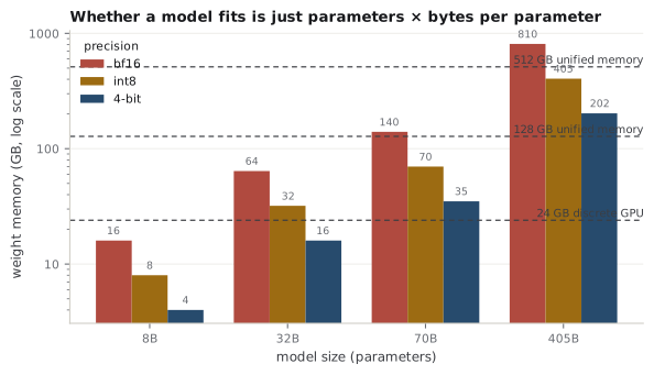
You also need headroom on top of the weights for two things: the KV cache, which grows with how much context you are holding, and a few gigabytes of runtime overhead. A practical rule is to leave 15–25% of memory free above the weight footprint.
A.2.1The KV cache
Every token you have already processed leaves behind a key and value vector in each layer, cached so you do not recompute it. Its size grows linearly with context length:
The factor of 2 is one each for keys and values. Note \(n_\text{kv\_heads}\), not the full head count: grouped-query attention (Chapter 5) shrinks this term deliberately, which is largely why it exists. For a mid-sized model at a long context the KV cache can rival the weights, so it is not a rounding error — it is often the reason a long prompt suddenly no longer fits.
A.3How fast? The bandwidth math
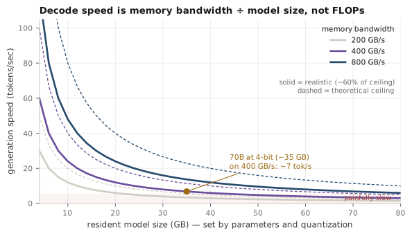
Here is the fact that surprises people: generating one token with a dense model requires reading every weight from memory once. Nothing clever avoids it — each new token's computation touches the whole network. So during generation (the decode phase, Chapter 15) you are limited not by how fast the chip computes but by how fast it can stream weights out of memory:
Intuition
Single-stream local generation is memory-bandwidth-bound, not compute-bound. The GPU spends most of its time waiting for weights to arrive, not multiplying. This is why "how many TFLOPs" matters far less than "how many GB/s" for local inference — and why quantizing a model makes it faster, not just smaller: fewer bytes per weight means fewer bytes to stream per token.
A worked example. Suppose a machine has 400 GB/s of memory bandwidth and you run a 70B model quantized to 4-bit (~35 GB):
Real throughput is perhaps 50–70% of that ceiling after overheads, so call it 6–8 tokens/sec — readable, roughly reading speed, but not instant. Halve the model with more aggressive quantization and you roughly double the rate.
Interview
Why does the same model run faster when quantized, beyond just fitting in memory? Because decode is memory-bandwidth-bound: throughput is (bandwidth ÷ bytes read per token). Fewer bits per weight means fewer bytes streamed per token, so tokens come out faster — the speedup is roughly proportional to the compression ratio, independent of the capacity savings.
Two nuances worth holding:
- Prefill vs decode. Processing your prompt (prefill) is compute-bound and parallel, so it is fast; generating the response (decode) is the bandwidth-bound part above. A long prompt with a short answer feels quick; a short prompt with a long answer is where you feel the tokens/sec.
- Batching does not help you locally. The bandwidth ceiling is generous when you serve many requests at once (you amortize each weight read across the batch), but a single user at a laptop runs batch size 1, so the ceiling above is what you get.
A.4Why Apple silicon is good at this
Discrete GPUs keep their fast memory (VRAM) separate from system RAM, and it is expensive and limited — a consumer card might have 24 GB, so a 70B model in 4-bit does not fit on one, and you are into multi-GPU territory with all its complexity.
Apple-silicon Macs use unified memory: the CPU and GPU share one large, high-bandwidth pool. There is no separate "VRAM" to run out of — the GPU can address all of system memory. So a Mac configured with, say, 128 GB of unified memory can hold models that would otherwise demand several discrete GPUs, and it does so with high bandwidth feeding the GPU cores directly.
Intuition
On a discrete GPU, capacity (VRAM) is the wall you hit first. On Apple silicon, capacity is generous because it is just system memory, so bandwidth becomes the thing that sets your token rate. Buy for the memory size that fits your target model, but understand that the memory bandwidth is what you will feel every time you generate.
On the hypothetical super-machine
If you are imagining a future high-memory Apple-silicon machine (an "M5"-class chip with a large unified-memory configuration and higher bandwidth than today's), the reasoning does not change — only the numbers do. Plug that machine's memory size into the capacity math to see which models fit, and its GB/s into the bandwidth math to predict tokens/sec. The framework is what matters; the spec sheet just fills in two variables.
A.5The tooling
You rarely implement any of this yourself. A few tools dominate local inference:
- llama.cpp — the C/C++ engine most local inference is built on. Runs the GGUF model format, which packages quantized weights with metadata, and supports Apple's Metal GPU backend. This is the layer doing the actual work.
- Ollama — a friendly wrapper over llama.cpp with a one-command model pull-and-run experience and a local API server. The easiest on-ramp.
- LM Studio — a desktop GUI over the same ecosystem, good for browsing and trying quantized models without the terminal.
- MLX — Apple's own array framework, built specifically for Apple silicon and unified memory. It is the path when you want to fine-tune or experiment (LoRA and friends, Chapter 13) on a Mac rather than only run inference, and it often gets the best performance on Apple hardware because it is tuned for exactly that chip.
Interview
What format and tool would you reach for to run a quantized model on a Mac, and why? A GGUF build of the model via llama.cpp (or Ollama on top of it) for inference, because it has mature Metal support and a wide catalog of ready-made quantizations; MLX if you also want to fine-tune, since it is written for Apple silicon's unified memory.
A.6A checklist
To decide if a model runs on a given machine:
- Capacity. Estimate weight memory as params × bytes-per-param at your chosen quantization; add a KV-cache allowance for your longest context; leave ~20% free. Does it fit in unified memory (or VRAM)?
- Speed. Divide the machine's memory bandwidth by the model size in bytes for a tokens/sec ceiling; expect to hit roughly half to two-thirds of it.
- Quantization. If it does not fit or is too slow, drop to a smaller quant (Q4 is the usual sweet spot for quality vs size) or a smaller model, and recompute.
Do those three and you can predict, before downloading a single gigabyte, whether a model will run well on your hardware.