6The Pretraining Objective and the Data
Part I froze the architecture; this part learns the weights. The objective could not be simpler — predict the next token, everywhere, on everything — and that simplicity moves all the leverage into two questions this chapter takes in turn: what the objective really optimizes, and what "everything" should be. The second question is the underrated one. Two teams with the same architecture and the same compute routinely get different models, and the difference is almost always the data.
6.1Next-token prediction as compression
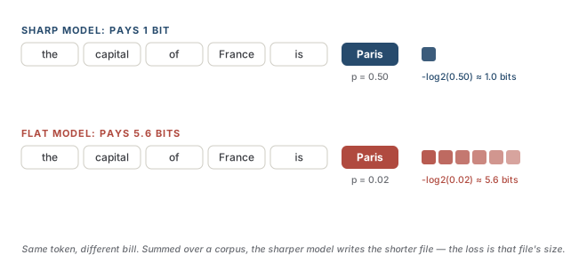
The training loss is cross-entropy: for each position, the negative log-probability the model assigned to the token that actually came next. Measured in base 2, that is literally a count of bits — and Chapter 1's perplexity is just this number re-expressed as a choice count. An old result gives the count an operational meaning: any probability distribution over the next symbol can drive an arithmetic coder that spends exactly \(-\log_2 p(x)\) bits encoding the symbol \(x\). A model that predicts well therefore is a compressor, mechanically, not metaphorically — and a strong LLM used this way out-compresses gzip on text by a wide margin (Delétang et al., 2024). Training to minimize cross-entropy is training to compress the corpus.
This is why "it just predicts the next token" is not the dismissal it sounds like. Shannon estimated English's entropy by having people play the guess-the-next-letter game, and found that guessing well requires knowing spelling, grammar, idiom, and context (Shannon, 1951). To compress arbitrary text toward its entropy, shallow statistics run out fast; the remaining bits are recoverable only from facts, structure, and reasoning. Compression pressure is what forces the model to learn them.
Intuition
A model that has to bet on every next token, on every text ever written, can only keep winning by understanding what the text is about. The loss is the bookkeeping of those bets, in bits.
Interview
Model A reports lower perplexity than model B — is A better? Only if they share a tokenizer. Perplexity is per token, and a tokenizer with a bigger vocabulary packs more text into each token, raising per-token entropy while compressing the sequence (Chapter 3). To compare across tokenizers, renormalize to bits per byte of raw text — the compression view again, which is tokenizer-independent.
The intuition has limits, and naming them is second-question territory. Prediction rewards matching the distribution of the corpus, including its errors, biases, and boilerplate; a perfect predictor of internet text confidently completes falsehoods that are common online. And the loss counts every token equally, though tokens differ wildly in how much they matter — getting a name or a digit wrong is billed the same one-token price as flubbing "the." What prediction alone cannot teach — that a prompt is a request from a user, not a document to continue — is Part III's opening problem.
6.2Where the data comes from
Scale first, because it sets the terms: modern pretraining corpora are measured in tokens, and the number has grown faster than model size. GPT-3 trained on roughly 300 billion tokens (Brown et al., 2020); Chinchilla made 1.4 trillion the compute-optimal choice for its size (Chapter 9 derives why) (Hoffmann et al., 2022); Llama 3 trained on about 15 trillion (Grattafiori et al., 2024). Counting in gigabytes misleads — deduplication, filtering, and tokenizer choice all change bytes-per-token — so the field standardized on the unit the loss actually consumes.
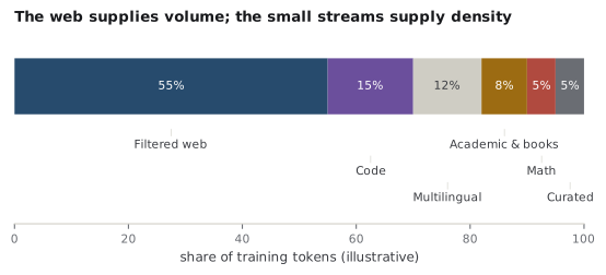
Where do trillions of tokens exist? Essentially one place: the web. Common Crawl, a nonprofit's ongoing scrape of the public internet, is the base ingredient of nearly every open corpus — The Pile drew on it alongside academic and specialist sources (Gao et al., 2020), and FineWeb refined roughly a hundred crawl snapshots into about 15 trillion usable tokens (Penedo et al., 2024). Around that base, every serious mixture adds smaller high-value streams: code (GitHub and its descendants), academic text (papers, textbooks), books, encyclopedic reference, math, and increasingly multilingual web. The web supplies volume; the curated streams supply density.
Note
Frontier labs disclose less about data than about anything else — data is where the competitive edge and the copyright exposure both live. The open-data projects (The Pile, FineWeb, and successors) are how the field actually knows what works.
6.3Cleaning and deduplication
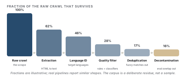
Raw crawl is unusable. It is boilerplate, navigation menus, SEO spam, auto-generated listings, adult content, and the same page mirrored ten thousand times. Between the crawl and the training run sits a pipeline that discards most of the internet:
- Extraction strips HTML to running text — an unglamorous step that changes downstream quality measurably (Penedo et al., 2024).
- Language identification routes documents to the intended language mix.
- Quality filtering drops junk, by hand-written heuristics (document length, symbol ratios, repetition) and by classifiers trained to score "does this look like text worth learning from."
- Deduplication removes exact and near-duplicate documents, typically with hash-based fuzzy matching at scale. Duplicated text distorts the implicit data mixture, wastes compute on repeats, and makes the model far more likely to memorize and regurgitate the repeated passage (Lee et al., 2022).
- Decontamination removes documents that overlap the evaluation benchmarks you intend to report. Test questions are on the internet too.
Common trap
Contamination does not just flatter a benchmark score; it silently converts an evaluation of generalization into an evaluation of recall, while the number still looks like the former. Chapter 24 returns to this from the evaluator's side — and to why decontamination by exact match is never fully clean, since paraphrases survive.
Each stage is a dial, not a switch, and the dials trade against each other: filter aggressively and you gain average quality but lose diversity and total tokens; filter lightly and you keep scale but learn spam. The striking empirical fact is how much these unglamorous choices matter — FineWeb's ablations show filtering and dedup decisions moving downstream benchmark accuracy by more than many architecture changes do (Penedo et al., 2024).
6.4Data mixtures and curriculum
Cleaned sources still have to be combined, and the weights are a first-class hyperparameter. Sampling proportionally to raw size would drown everything in web text, so high-density domains are upsampled — a small math corpus might be repeated several times per "epoch" of web text. Repetition is affordable in moderation: up to roughly four epochs over a source costs little versus fresh data, after which returns decay sharply (Muennighoff et al., 2023). Tuning the weights by grid search is hopeless at full scale, so mixtures are tuned on small proxy runs, or learned — DoReMi trains a small model to find domain weights that transfer to a much larger run (Xie et al., 2023).
Code deserves its own sentence: every modern mixture over-weights it, even for models not aimed at programmers, because training on code measurably improves structured, multi-step behavior in prose — it is the largest corpus of explicit logical procedure ever written.
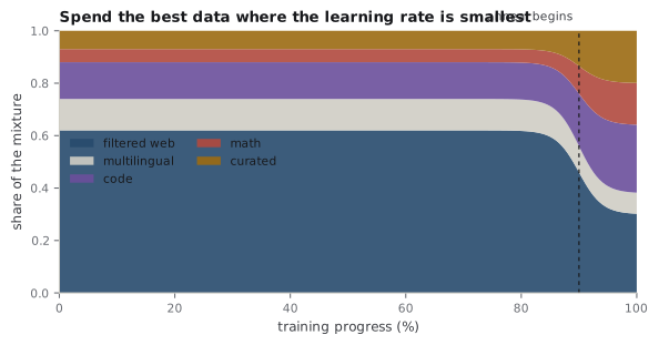
The mixture also need not be constant. The most common curriculum is annealing: in the final stretch of training, as the learning rate decays toward zero (Chapter 7), the mixture shifts toward the highest-quality sources — curated text, math, code (Grattafiori et al., 2024; Hu et al., 2024). The last tokens a model sees under a tiny learning rate are the ones that most directly shape its final polish, so you spend your scarcest, best data there.
Analogy
It is exam-week studying: a semester of broad reading, then the final days spent only on the best notes. The analogy leaks in one way — the model does not consolidate on its own between sessions; the annealing schedule has to be the consolidation, which is why its placement against the learning-rate decay matters.
Interview
You have a fixed token budget and your model underperforms on reasoning. What is the cheapest lever? Not architecture — mixture. Upweight code and math, consider a quality-filtered second pass on the best web data, and anneal on your highest-quality sources at the end of training. Data interventions dominate architecture interventions at fixed compute, which is why data work is where pretraining teams actually spend their time.
The objective and the diet are set. What remains is to actually run the loop from Chapter 2 a few million times without it exploding — the subject of the next chapter.
References
- Brown, T., Mann, B., Ryder, N., Subbiah, M., et al. (2020). Language models are few-shot learners. Advances in Neural Information Processing Systems. arXiv:2005.14165.
- Delétang, G., Ruoss, A., Duquenne, P.-A., Catt, E., et al. (2024). Language modeling is compression. International Conference on Learning Representations. arXiv:2309.10668.
- Gao, L., Biderman, S., Black, S., Golding, L., et al. (2020). The Pile: An 800GB dataset of diverse text for language modeling. arXiv preprint. arXiv:2101.00027.
- Grattafiori, A., Dubey, A., Jauhri, A., Pandey, A., et al. (2024). The Llama 3 herd of models. arXiv preprint. arXiv:2407.21783.
- Hoffmann, J., Borgeaud, S., Mensch, A., Buchatskaya, E., et al. (2022). Training compute-optimal large language models. Advances in Neural Information Processing Systems. arXiv:2203.15556.
- Hu, S., Tu, Y., Han, X., He, C., et al. (2024). MiniCPM: Unveiling the potential of small language models with scalable training strategies. arXiv preprint. arXiv:2404.06395.
- Lee, K., Ippolito, D., Nystrom, A., Zhang, C., et al. (2022). Deduplicating training data makes language models better. Association for Computational Linguistics. arXiv:2107.06499.
- Muennighoff, N., Rush, A. M., Barak, B., Le Scao, T., et al. (2023). Scaling data-constrained language models. Advances in Neural Information Processing Systems. arXiv:2305.16264.
- Penedo, G., Kydlíček, H., Ben Allal, L., Lozhkov, A., et al. (2024). The FineWeb datasets: Decanting the web for the finest text data at scale. Advances in Neural Information Processing Systems (Datasets and Benchmarks). arXiv:2406.17557.
- Shannon, C. E. (1951). Prediction and entropy of printed English. Bell System Technical Journal, 30(1).
- Xie, S. M., Pham, H., Dong, X., Du, N., et al. (2023). DoReMi: Optimizing data mixtures speeds up language model pretraining. Advances in Neural Information Processing Systems. arXiv:2305.10429.
Check yourself
Interview-style questions on this chapter. Pick an answer to see whether it holds up.
-
Model A (32k-token vocabulary) reports perplexity 9; model B (128k-token vocabulary) reports perplexity 12 on the same text. What can you conclude about which predicts the text better?
A tokenizer choice changes the unit of measurement. Each of B's tokens carries more text, so its per-token perplexity is naturally higher even if it compresses the text better overall. Converting both models' total cross-entropy to bits per byte of the same underlying text removes the tokenizer from the comparison - which is exactly the compression view of the loss. -
Beyond wasting compute on repeats, why does deduplication measurably improve a pretrained model?
Lee et al. (2022) showed near-duplicate text both skews the effective data distribution and drives verbatim memorization, which is a privacy and quality problem. Dedup reduces memorization sharply but does not eliminate it - unique text seen once can still be memorized, especially by large models late in training. -
Why do pretraining teams shift the data mixture toward their highest-quality sources specifically during the final learning-rate decay, rather than spreading that data evenly?
Annealing pairs the mixture shift with the learning-rate decay deliberately: nothing comes after the anneal to disturb what it teaches. Llama 3 and MiniCPM both report this recipe. It is also why a mid-training checkpoint understates final model quality - the anneal's gains have not happened yet. -
Your corpus is short of fresh tokens for the planned run. What does the evidence on repeating data say?
Muennighoff et al. (2023) fit scaling laws in the data-constrained regime: a few epochs are nearly as good as unique tokens, then value decays sharply. This is why small high-quality sources are routinely upsampled several times per web epoch, and why the 'running out of data' question is about fresh-token supply, not literal exhaustion. -
What is the precise sense in which a language model 'is' a compressor?
The equivalence is mechanical, not metaphorical: any predictor plus arithmetic coding is a lossless compressor, and the achieved file size is the model's cross-entropy on that text. Deletang et al. (2024) demonstrate strong LLMs out-compressing gzip this way. The weights-are-smaller-than-the-data reading is a looser, different claim - the coding argument is the one to give in an interview.