15Making Inference Fast
A trained model is not fast or slow on its own; how you run it decides. This chapter is organized around a single fact that shapes every technique in it: generating text is bottlenecked by memory bandwidth, not arithmetic. The GPU can multiply far faster than it can fetch the numbers to multiply, so the game at inference time is to move fewer bytes and to do more useful work per byte moved. Read prefill-versus-decode, the KV cache, batching, speculation, and FlashAttention as five different answers to that one problem.
15.1Prefill and decode are two different machines
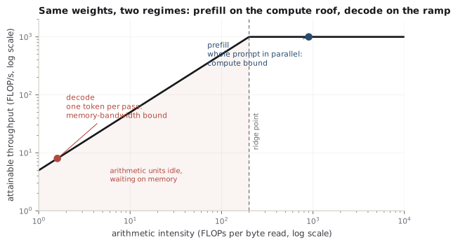
Serving a request splits into two phases with opposite characters. Prefill reads the whole prompt at once: every prompt token flows through the model in parallel, in one big batched matrix multiply, exactly like a training forward pass. Decode then generates the answer one token at a time, and each step must run a full forward pass to produce a single new token before it can even begin the next.
The difference that matters is arithmetic intensity — floating-point operations performed per byte read from memory. Prefill reuses each weight across all the prompt's tokens, so it does a lot of math per byte and saturates the GPU's arithmetic units: it is compute-bound. Decode reads the entire model — every weight, plus the growing KV cache — to compute one token, so it does almost no math per byte and the arithmetic units sit idle waiting on memory: it is memory-bandwidth-bound. This is the same wall Appendix A hits from the hardware side, where generation speed came out as bandwidth divided by model size.
Intuition
Prefill is reading a page you already have; decode is writing the next word, then walking back to re-read the entire book before writing the word after that. The reading dominates, and it is reading from slow memory.
Because prefill happens once but decode runs once per output token, end-to-end speed on any nontrivial generation is dominated by decode. That is why almost everything downstream — batching, the KV cache, quantization (Chapter 16) — is really about making the memory-bound decode phase move fewer bytes.
Interview
A serving team reports two latency numbers, TTFT and TPOT — what are they measuring? Time-to-first-token is prefill: how long until the prompt is processed and the first token appears. Time-per-output-token is decode: the steady-state cost of each subsequent token, set by memory bandwidth. They trade off differently, which is why serving systems (Chapter 17) schedule the two phases separately.
15.2The KV cache turns recomputation into memory
Attention at position \(t\) needs the keys and values of every earlier token. Naively, generating each new token would recompute the keys and values for the entire prefix, making generation cost grow with the square of the sequence — the \(O(n^2)\) of Chapter 4, paid again at every step. The KV cache removes that: keys and values, once computed, are stored and reused, so each decode step computes the K and V for only the one new token and reads the rest from the cache.
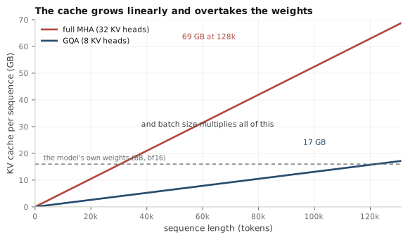
The catch is that you have traded compute for memory, and that memory grows. The cache holds, for every layer and every past token, one key vector and one value vector:
The leading 2 is keys and values; it grows linearly in both sequence length and batch size. Work it out for a Llama-3-8B-class model (32 layers, 8 KV heads, head dimension 128, bf16): about 128 KB per token, so a single 128k-token context holds roughly 16 GB of cache — comparable to the 16 GB of weights themselves. Multiply by batch size and the cache, not the weights, is what fills the GPU and caps how many requests you can serve at once.
Interview
Why does a long context slow decoding down even after prefill is done? Because every decode step streams the whole KV cache out of memory to attend over it, and the cache grows with context length. Decode is bandwidth-bound, so a bigger cache means more bytes per token means fewer tokens per second — the cost of long context is paid on every single step, not just once at prefill.
This is exactly why the attention variants of Chapter 5 exist. Grouped-query and multi-query attention shrink \(n_{\text{kv}}\) directly (Ainslie et al., 2023; Shazeer, 2019); sliding-window attention caps the effective sequence length (Jiang et al., 2023); multi-head latent attention compresses K and V into a small shared latent (DeepSeek-AI, 2024). Quantizing the cache to fewer bytes per entry (Chapter 16) is a fourth lever. All four attack the same term in the formula above.
15.3Batching and PagedAttention
Since decode re-reads the weights for every token, the way to get throughput is to make each read count for more: batch requests so one weight-read serves many sequences at once. Batching is the single biggest throughput lever precisely because it amortizes the memory-bound decode over more useful work.
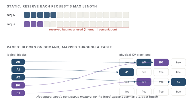
Naive static batching wastes most of that promise. Requests in a batch finish at different times, so a batch sized for the slowest request leaves the rest idling; worse, each sequence needs contiguous KV memory reserved for its maximum possible length, most of which is never used. The result is severe internal fragmentation and small effective batches. Two ideas fix it. Continuous (in-flight) batching swaps finished sequences out and new ones in at the granularity of individual tokens, keeping the batch full (its origin, Orca, is Chapter 17's to develop). And PagedAttention solves the memory side by borrowing the operating system's oldest trick (Kwon et al., 2023).
Analogy
PagedAttention treats KV memory the way an OS treats RAM: split it into fixed-size blocks, hand them out on demand, and keep a per-sequence block table mapping a request's logical blocks to scattered physical ones. A sequence never needs contiguous space, so fragmentation nearly vanishes and shared prefixes can share physical blocks copy-on-write. The analogy leaks in that KV blocks are only ever appended to, never randomly written, so there is no true page-replacement policy — nothing gets swapped to disk mid-attention.
The payoff is concrete: vLLM's paged cache raised serving throughput several-fold over contiguous allocation at the same latency, by fitting far larger batches into the same memory (Kwon et al., 2023). Paging is now standard in every serious inference engine.
15.4Speculative decoding buys parallelism back
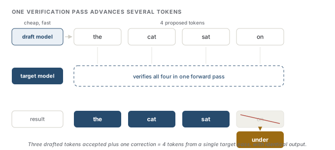
Decode is slow because it is sequential: one forward pass per token, each waiting on the last. Speculative decoding breaks that dependency with a bet. A small, cheap draft model proposes the next few tokens quickly; the large target model then verifies all of them in a single forward pass, checking each proposed token against what it would have produced (Leviathan et al., 2023; Chen et al., 2023). Verifying \(k\) tokens at once is a parallel, prefill-like operation, so it is nearly as cheap as generating one — and the target had spare compute to burn, being memory-bound. Accept the longest correct prefix, resample the first wrong token, and repeat.
The remarkable part is that this is exact. A carefully constructed rejection-sampling step makes the output distribution identical to sampling from the target alone — you get the same tokens the big model would have produced, using fewer of its forward passes (Leviathan et al., 2023). That is the free-lunch intuition: no quality cost, only fewer expensive steps.
Intuition
The draft model does the easy guessing; the big model just grades the guesses, and grading a whole batch of them costs about as much as producing one. When the guesses are mostly right, you advance several tokens per expensive step.
The lunch is not unconditional. The speedup is the expected number of accepted tokens per verification, which depends on the acceptance rate — how often the draft agrees with the target — and on the draft being genuinely cheap. A weak draft gets rejected constantly and you pay its cost for little gain; too strong a draft is slow enough to erase the win. Acceptance also collapses on hard or high-entropy text where even the target is unsure. A popular variant removes the separate draft entirely: Medusa and other self-speculation methods bolt extra decoding heads onto the target model itself to predict several tokens ahead, then verify with tree attention (Cai et al., 2024).
15.5FlashAttention moves less memory, not fewer FLOPs
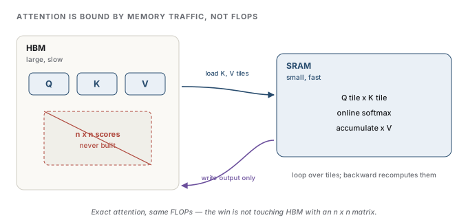
The last lever returns to Chapter 4's \(O(n^2)\) and reads it correctly. The quadratic cost is real, but a standard attention implementation is slow for a subtler reason: it builds the full \(n \times n\) score matrix in the GPU's large, slow memory (HBM), writes it out, reads it back to apply softmax, and reads it yet again to multiply by the values. Attention is dominated by that memory traffic, not by the arithmetic.
FlashAttention is IO-aware: it computes the exact same attention without ever materializing the score matrix (Dao et al., 2022). It tiles Q, K, and V into blocks small enough to fit in the GPU's fast on-chip memory (SRAM), and streams over them, maintaining a running "online" softmax that updates the output block by block. Nothing \(n \times n\) is ever written to HBM; on the backward pass it recomputes the needed blocks rather than storing them, trading a little extra arithmetic for a large cut in memory traffic.
Common trap
FlashAttention does not reduce the FLOP count — it does the same (or slightly more) arithmetic. It is faster because attention was memory-bound, so cutting HBM reads and writes is what actually moves the clock. Calling it an "approximation" or a "lower-complexity attention" is the giveaway that a candidate has the mental model wrong: it is exact, and still \(O(n^2)\) in compute.
The follow-on FlashAttention-2 rebalances the work across the GPU's thread blocks and warps to keep more of the hardware busy, closing much of the remaining gap to peak (Dao, 2023); later versions specialize further for newer accelerators. All of them are the same idea: keep the working set in fast memory and never spill the big matrix.
Together these techniques decide what a model costs to run. The next chapter cuts the bytes themselves with quantization (Chapter 16), and Chapter 17 assembles all of it into a production serving stack.
References
- Ainslie, J., Lee-Thorp, J., de Jong, M., Zemlyanskiy, Y., Lebrón, F., & Sanghai, S. (2023). GQA: Training generalized multi-query transformer models from multi-head checkpoints. Empirical Methods in Natural Language Processing. arXiv:2305.13245.
- Cai, T., Li, Y., Geng, Z., Peng, H., et al. (2024). Medusa: Simple LLM inference acceleration framework with multiple decoding heads. International Conference on Machine Learning. arXiv:2401.10774.
- Chen, C., Borgeaud, S., Irving, G., Lespiau, J.-B., Sifre, L., & Jumper, J. (2023). Accelerating large language model decoding with speculative sampling. arXiv preprint. arXiv:2302.01318.
- Dao, T., Fu, D. Y., Ermon, S., Rudra, A., & Ré, C. (2022). FlashAttention: Fast and memory-efficient exact attention with IO-awareness. Advances in Neural Information Processing Systems. arXiv:2205.14135.
- Dao, T. (2023). FlashAttention-2: Faster attention with better parallelism and work partitioning. arXiv preprint. arXiv:2307.08691.
- DeepSeek-AI (2024). DeepSeek-V2: A strong, economical, and efficient mixture-of-experts language model. arXiv preprint. arXiv:2405.04434.
- Jiang, A. Q., Sablayrolles, A., Mensch, A., Bamford, C., et al. (2023). Mistral 7B. arXiv preprint. arXiv:2310.06825.
- Kwon, W., Li, Z., Zhuang, S., Sheng, Y., et al. (2023). Efficient memory management for large language model serving with PagedAttention. ACM Symposium on Operating Systems Principles (SOSP). arXiv:2309.06180.
- Leviathan, Y., Kalman, M., & Matias, Y. (2023). Fast inference from transformers via speculative decoding. International Conference on Machine Learning. arXiv:2211.17192.
- Shazeer, N. (2019). Fast transformer decoding: One write-head is all you need. arXiv preprint. arXiv:1911.02150.
Check yourself
Interview-style questions on this chapter. Pick an answer to see whether it holds up.
-
A model generates at only a few tokens per second on a GPU whose arithmetic units are nearly idle, yet the same GPU processes a long prompt almost instantly. What explains the gap?
The two phases have opposite arithmetic intensity. Prefill reuses each weight across all prompt tokens at once, saturating the arithmetic units; decode reads the whole model (and KV cache) to emit a single token, so it is limited by how fast memory can be read, not by FLOPs. This is why generation speed tracks memory bandwidth divided by model size, and why the arithmetic units sit idle during decode. -
Why does serving a 128k-token context slow down every decode step, not just the initial prefill?
Decode is memory-bandwidth-bound, and the KV cache is memory that must be read on every step. Its size grows linearly with sequence length (and batch), so long context raises the per-token byte count for the whole generation, not once. The cache — not the weights — is usually what caps context length and batch size, which is why GQA, sliding windows, and MLA all target its size. -
PagedAttention is often summarized as 'virtual memory for the KV cache.' What concrete problem does it actually solve?
Static allocation reserves contiguous memory for each request's worst-case length, most of which goes unused — severe internal fragmentation that shrinks the batch. PagedAttention allocates small blocks on demand and maps logical to physical blocks through a per-sequence block table, so no request needs contiguous space and shared prefixes can share blocks. The freed memory becomes a larger batch, which is the throughput win — it does not compress or swap the cache. -
In speculative decoding a small draft model proposes tokens that a large target verifies. A candidate calls it 'an approximation that trades a little quality for speed.' What is wrong with that?
Speculative decoding is exact. The acceptance test plus resampling of the first rejected token provably reproduce the target's own distribution, so the generated text is what the target would have produced. The benefit is doing several tokens' worth of progress per expensive target pass, since verifying k proposed tokens is a parallel, prefill-like operation on a target that had spare compute. -
You add speculative decoding with a strong, accurate draft model and see almost no speedup. What is the most likely reason?
The speedup is roughly the expected accepted tokens per step divided by the combined draft-plus-target cost. A draft strong enough to be accurate is often nearly as expensive as the target, so you pay almost a full model per proposed token and the arithmetic stops favoring you. The sweet spot is a draft that is both cheap and reasonably aligned — high acceptance is only half the equation. -
FlashAttention is frequently described as making attention 'cheaper.' What does it actually reduce, and why is that the thing that matters?
FlashAttention is exact and still O(n-squared) in compute; it does the same (or slightly more) arithmetic. Standard attention is slow because it materializes and re-reads the n-by-n score matrix in HBM, and attention is memory-bound. Tiling Q, K, and V through SRAM with an online softmax cuts that traffic, and recomputing tiles in the backward pass avoids storing the matrix at all. The win is bytes moved, not FLOPs — the same reason decode is slow in the first place.