8Distributed Training

Distributed training sounds like an infrastructure appendix, but it is where interviews reliably go deep, and it runs on one plain idea: a model's training state is too big for any single device, so you must decide what to replicate and what to shard — and every choice buys memory with communication. This chapter builds the standard answers in the order teams reach for them: shard the optimizer, then split the layers, then split the stack, then compose all three; and it ends with the communication primitives that decide what any of it costs.

8.1Why one GPU is never enough

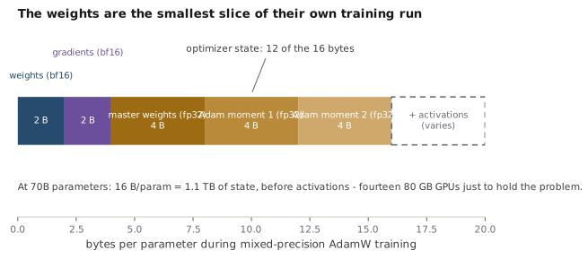
Chapter 2's interview question established that training holds far more than weights. Make it concrete with mixed-precision AdamW, per parameter: bf16 weights (2 bytes) and gradients (2 bytes), plus an fp32 master copy of the weights (4) and Adam's two moments (4 + 4) — 16 bytes per parameter before a single activation is stored. A 70B-parameter model therefore carries about 1.1 TB of training state against an 80 GB accelerator: fourteen devices just to hold the problem, before the batch's activations — which scale with batch size, sequence length, and depth, and at long context can rival the fixed state — claim their share.

Notice the villain ranking: the optimizer state (12 of the 16 bytes) dwarfs the weights you actually wanted. That single observation motivates the entire next section.

8.2Data parallelism and ZeRO/FSDP

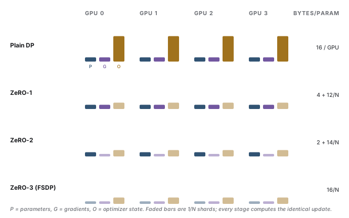
Data parallelism (DP) is the default: copy the full model to every GPU, give each a different slice of the batch, and after the backward pass all-reduce the gradients so every copy takes the identical optimizer step. Compute scales beautifully. Memory does not improve at all — every GPU still holds all 16 bytes per parameter, so plain DP cannot train a model that does not already fit.

ZeRO's observation is that the replication is redundant (Rajbhandari et al., 2020): across \(N\) data-parallel GPUs, there is no reason to keep \(N\) identical copies of state that could be split \(N\) ways. Its three stages form a memory ladder, each rung shard­ing the next-largest tenant:

1. Stage 1 shards the optimizer state (the 12-byte villain). Each GPU updates only its shard of the parameters.
2. Stage 2 also shards the gradients: instead of all-reducing full gradients, each GPU receives only the reduced gradient for its own shard (a reduce-scatter).
3. Stage 3 also shards the parameters themselves. Nothing is replicated; each layer's weights are all-gathered just in time for its forward or backward pass, used, and discarded.

Stage 3 is what PyTorch ships as FSDP — fully sharded data parallel (Zhao et al., 2023). Per-GPU memory falls almost \(N\)-fold, at the price of moving parameters over the wire every step; the arithmetic of whether that price is payable is the interconnect question the last section answers.

8.3Tensor and pipeline parallelism

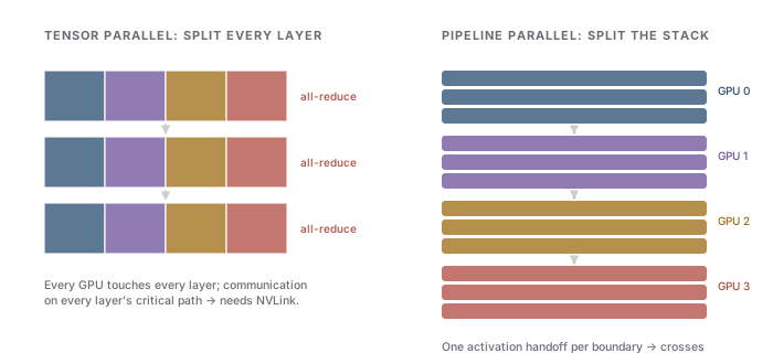
ZeRO shards storage but still runs every layer's full computation on each GPU. The model-parallel families split the computation itself, along two orthogonal cuts.

Tensor parallelism (TP) slices within a layer (Shoeybi et al., 2019). A weight matrix is split column-wise across GPUs; each computes its slice of the matmul, and an all-reduce reassembles the result. Megatron's arrangement needs only two all-reduces per transformer block by pairing a column-split matrix with a row-split one — but those all-reduces sit on the critical path of every layer, every microbatch. TP is therefore chatty and latency-sensitive, and in practice lives only inside a node, where NVLink-class bandwidth makes the chatter affordable.

Pipeline parallelism (PP) slices between layers (Huang et al., 2019): GPU 0 takes blocks 1–8, GPU 1 takes 9–16, and activations flow stage to stage. Communication is tiny — one activation tensor per boundary — so pipelines happily cross nodes. The tax is the bubble: stage \(k\) idles until work reaches it, and idles again as the pipeline drains. The fix is to chop the batch into \(m\) microbatches so stages overlap; with \(p\) stages the idle fraction is roughly \((p-1)/(m+p-1)\), which is why pipeline configurations always come with large microbatch counts and why deeper pipelines demand them.

8.4Putting it together: 3D parallelism

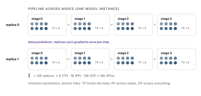
The three parallelisms answer different constraints, so frontier training uses all of them at once (Narayanan et al., 2021), and the composition follows the hardware's own hierarchy:

• TP spans the GPUs within one node, where bandwidth is highest — typically 8.
• PP spans nodes, because stage boundaries tolerate slower links — say 16 stages.
• DP (with ZeRO sharding as needed) replicates that whole 128-GPU model instance and splits the global batch across replicas.

The back-of-envelope for a Llama-3-405B-class run (Grattafiori et al., 2024): \(8 \text{ (TP)} \times 16 \text{ (PP)} = 128\) GPUs to hold one model instance, times \(128\) data-parallel replicas \(= 16{,}384\) GPUs, with the global batch divided among replicas and each replica's share divided into microbatches to keep its pipeline full. Long-context training adds a fourth axis (splitting the sequence itself), and mixture-of-experts models add expert parallelism (Chapter 5) — but every axis is still the same one decision, replicate or shard, applied to a different dimension of the problem.

8.5The communication primitives

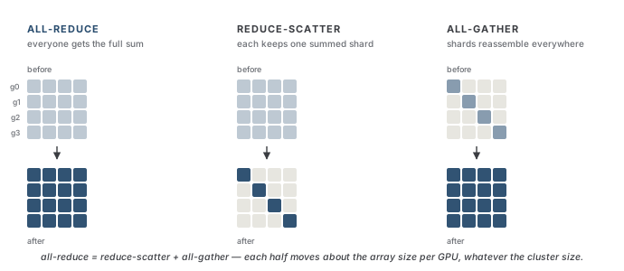
Every scheme above reduces to three collective operations, and knowing them turns hand-waving into arithmetic:

• All-reduce: every GPU contributes an array; every GPU ends with the elementwise sum. Data parallelism's gradient sync.
• Reduce-scatter: the same sum, but each GPU keeps only its \(1/N\) shard of the result. ZeRO-2's gradient move.
• All-gather: each GPU contributes a shard; every GPU ends with the concatenation. How ZeRO-3/FSDP rematerializes parameters.

The identity worth memorizing: all-reduce = reduce-scatter + all-gather. Ring implementations of the halves each move about \((N-1)/N\) of the data volume per GPU — near bandwidth-optimal, and nearly independent of \(N\) — so an all-reduce costs roughly \(2\times\) the array size in traffic per GPU, whatever the cluster size. ZeRO's stages are not exotic protocols; they are the two halves of the all-reduce DP already performed, with storage rearranged between them.

That constant factor is why interconnect bandwidth is destiny. The traffic per step is fixed by model size and parallelism layout; the wall-clock it costs is that traffic divided by link speed — and the links span orders of magnitude, from NVLink-class intra-node fabric (hundreds of GB/s per GPU) to inter-node InfiniBand (tens). Whether communication hides behind computation or dominates it is decided by which link each collective runs over; that is the entire content of the placement rules above, and it is why clusters are bought around their network as much as their FLOPs. The same bandwidth obsession returns at serving time (Chapter 15), where the wire is replaced by GPU memory itself.

With the machinery to hold and feed a model at any size, one question is left hanging over Part II: how big should the model be, and how many tokens should it eat? That question turns out to have an equation.

References

- Grattafiori, A., Dubey, A., Jauhri, A., Pandey, A., et al. (2024). The Llama 3 herd of models. arXiv preprint. arXiv:2407.21783.
- Huang, Y., Cheng, Y., Bapna, A., Firat, O., et al. (2019). GPipe: Efficient training of giant neural networks using pipeline parallelism. Advances in Neural Information Processing Systems. arXiv:1811.06965.
- Narayanan, D., Shoeybi, M., Casper, J., LeGresley, P., et al. (2021). Efficient large-scale language model training on GPU clusters using Megatron-LM. International Conference for High Performance Computing, Networking, Storage and Analysis (SC21). arXiv:2104.04473.
- Rajbhandari, S., Rasley, J., Ruwase, O., & He, Y. (2020). ZeRO: Memory optimizations toward training trillion parameter models. International Conference for High Performance Computing, Networking, Storage and Analysis (SC20). arXiv:1910.02054.
- Shoeybi, M., Patwary, M., Puri, R., LeGresley, P., Casper, J., & Catanzaro, B. (2019). Megatron-LM: Training multi-billion parameter language models using model parallelism. arXiv preprint. arXiv:1909.08053.
- Zhao, Y., Gu, A., Varma, R., Luo, L., et al. (2023). PyTorch FSDP: Experiences on scaling fully sharded data parallel. Proceedings of the VLDB Endowment, 16(12). arXiv:2304.11277.
Check yourself
Interview-style questions on this chapter. Pick an answer to see whether it holds up.
-
In mixed-precision AdamW training, roughly how do the 16 bytes per parameter break down, and what does that imply about what to shard first?
The counterintuitive headline is that the weights are the smallest tenant of their own training run: master weights (4) plus two moments (4+4) make the optimizer state six times the bf16 weights. Sharding it across N data-parallel workers (ZeRO-1) removes most of the redundancy without adding communication to the layer-by-layer critical path. -
A colleague worries that switching from plain data parallelism to ZeRO-3/FSDP will change the model's training trajectory. What is the correct response?
ZeRO's insight is that N data-parallel replicas hold N identical copies of state that can be split N ways and reassembled on demand (all-gather for parameters, reduce-scatter for gradients). The arithmetic is unchanged; only where the bytes live changes. That is what separates it from tensor or pipeline parallelism, which restructure the computation itself. -
Why does tensor parallelism stay within a single node while pipeline parallelism crosses nodes?
The placement rule is: match communication appetite to link speed. TP is chatty and latency-sensitive (per-layer, per-microbatch), PP is quiet (per-boundary), and DP syncs once per step and overlaps with compute. Inverting the order - TP across slow links - stalls every layer of every forward and backward pass. -
A pipeline has p stages and processes m microbatches per step. What fraction of time is lost to the bubble, and what follows from the formula?
While the pipeline fills and drains, early and late stages idle; with m microbatches in flight the overhead amortizes as (p-1)/(m+p-1). Doubling pipeline depth without doubling microbatches lowers utilization - one reason batch sizes at scale are large, and why pipeline schedules (interleaving, one-forward-one-backward) are an active engineering area. -
Why is 'all-reduce = reduce-scatter + all-gather' more than trivia?
Ring implementations of each half move (N-1)/N of the data per GPU - nearly constant in N - which makes communication budgets predictable and explains why ZeRO-2's traffic matches plain DP's. The identity turns 'exotic sharding scheme' into 'the same two collectives, reordered', which is the level of understanding interviews probe for.