Chapter 9

9Scaling Laws

Chapter 1 promised that scaling laws are the closest thing the field has to a design equation. Here is the claim in full: the pretraining loss of a language model is predictable — from model size, data size, and compute — by simple power laws that hold across many orders of magnitude. That regularity is why anyone dares spend nine figures on a single run: the loss of the big model is forecast from a fleet of cheap small ones. This chapter covers the laws, the correction that reshaped the field's budgets, the serving-cost amendment that reshaped them again, and the honest boundary of what the laws can promise.

9.1The empirical power laws

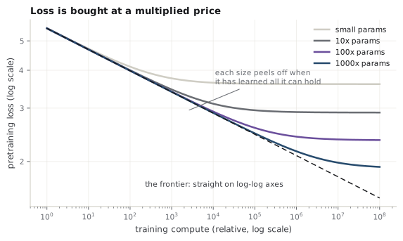
Train a family of models, varying one ingredient at a time with the others kept ample, and the pretraining loss \(L\) falls as a power law in each: in parameter count \(N\), in dataset size \(D\), and in training compute \(C\) (Kaplan et al., 2020). Power laws are straight lines on log-log axes, and their exponents are small — for compute, roughly \(L \propto C^{-0.05}\) — which packs the whole economics of the field into one shape: progress never stops, and every further increment costs about ten times more than the last. Two details of the Kaplan et al. findings carry the weight:

The law is astonishingly stable. It holds over many orders of magnitude with no visible bend, which is what makes extrapolation — the whole point — trustworthy enough to bet a datacenter on.
Shape barely matters; scale does. At fixed parameter count, depth-versus-width choices shift the loss only slightly. Within the transformer family, how big beats how shaped — the empirical license for Chapter 5's conservatism about architecture.

The loss being predicted also has a floor: fitted laws include an irreducible term, the entropy of text itself (Chapter 6's compression view says why — even a perfect model cannot spend fewer bits than the text truly contains). Scaling buys the reducible part.

Intuition

A scaling law is a price list, not a speedometer. It does not say models improve over time; it says exactly what a given loss costs in compute — and that each next increment of quality is bought at a multiplied price.

Training curves for a family of model sizes on log-log axes of compute and loss; each model peels off the shared frontier when it saturates, and the frontier itself is a straight line. — Figure 9.1The design equation. Each model size rides the same frontier and peels off when it has learned all it can hold; the frontier is a straight line on log-log axes across many orders of magnitude. Forecasting a frontier run means extending this line — which is exactly how the big bets are justified.

9.2Compute-optimal training: Chinchilla

A budget question follows immediately: given a fixed compute budget \(C\), and the serviceable approximation \(C \approx 6ND\) (six floating-point operations per parameter per training token), how should you split it between model size \(N\) and tokens \(D\)? Kaplan's fit said to grow \(N\) much faster than \(D\), and the field obeyed — GPT-3 put 175B parameters on 300B tokens (Brown et al., 2020).

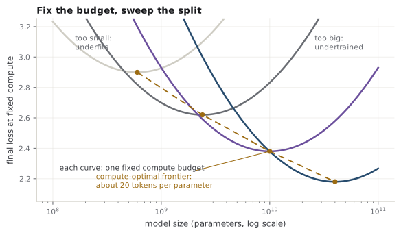
The Chinchilla work rechecked the fit and found a confound: the small-model runs had used a learning-rate schedule mismatched to their length, understating what small models achieve when properly trained (Chapter 7's cosine must land at the final token) (Hoffmann et al., 2022). Redone with matched schedules — including isoFLOP sweeps that train many \((N, D)\) pairs at the same total compute and locate the loss minimum — the answer changed to: scale \(N\) and \(D\) in equal proportion, roughly 20 tokens per parameter at the optimum. GPT-3-era models were several-fold undertrained: too many parameters, too few tokens. The demonstration was a 70B model trained on 1.4T tokens that outperformed models four times its size trained on the same compute (Hoffmann et al., 2022).

Common trap

"Chinchilla-optimal" does not mean 20 tokens per parameter is the right way to train. It answers one narrow question — the best loss for a fixed training budget, with everything after training priced at zero. Change the question and the answer moves; the next section changes the question.

Several U-shaped isoFLOP curves, each plotting loss against model size at one fixed compute budget; the minima drift diagonally, tracing the compute-optimal frontier where parameters and tokens grow in equal proportion. — Figure 9.2The isoFLOP argument. Fix a compute budget, sweep model size against it (bigger model, fewer tokens), and the loss is U-shaped: too small underfits, too large undertrains. The minima across budgets trace the compute-optimal path — about twenty tokens per parameter.

9.3Inference-aware scaling

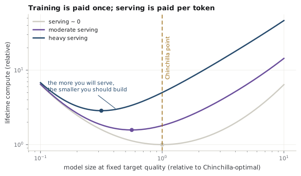
Chinchilla's accounting stops at the end of training, but a deployed model's life is mostly after that: every parameter is paid for again on every token it ever serves (Chapter 15 details the memory-bandwidth bill). Fold lifetime inference into the objective and the optimum shifts, in one direction only: smaller model, more tokens (Sardana et al., 2024). Training past the Chinchilla point wastes training compute in exchange for reaching a target quality in fewer parameters — and if the model will serve billions of requests, that trade pays for itself indefinitely.

This is not a theoretical refinement; it is the visible strategy of the entire open-weight era. Llama trained 7B-class models far past "optimal" precisely because they had to run on modest hardware (Touvron et al., 2023), and Llama 3 pushed its 8B model to 15T tokens — nearly 1,900 tokens per parameter, two orders of magnitude past the Chinchilla ratio, with the loss still improving (Grattafiori et al., 2024). A frontier lab serving hundreds of millions of users faces the same arithmetic at a different scale, which is why overtrained-small became the industry's default shape and pure Chinchilla-optimal training a niche.

Interview

Llama 3 8B trained on about 1,900 tokens per parameter. Is that a mistake by the Chinchilla rule? No — it is a different objective. Chinchilla minimizes loss for a fixed training budget; Llama minimizes lifetime cost, where every serving token re-pays the parameter count. Overtraining deliberately overspends on training to buy a smaller model that is cheaper at inference forever. The strong answer names the regime change: training cost is paid once, serving cost is paid per token.

Total lifetime compute versus model size at a fixed target quality, for three inference volumes; with negligible serving the optimum sits at the Chinchilla point, and as lifetime tokens grow the optimum slides toward smaller, longer-trained models. — Figure 9.3The amendment that runs the industry. At a fixed target quality, add lifetime serving cost to the training bill and the optimal model shrinks — the more tokens you will ever serve, the further past Chinchilla you should train. Every parameter is paid for once in training and forever after in serving.

9.4What scaling laws do and don't predict

Everything above predicts one number: next-token loss on the training distribution. The gap between that number and what anyone actually cares about is where scaling-law claims go wrong, and it has three parts.

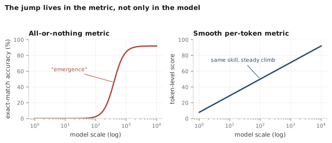
Loss is not capability. Downstream abilities can appear abruptly with scale even as the loss falls smoothly (Wei et al., 2022) — though Chapter 1's interview box carries the counterpoint that much of the abruptness is manufactured by all-or-nothing metrics (Schaeffer et al., 2023). The two views agree on what matters here: per-task forecasting from the loss curve is unreliable in both directions. The law tells you the big run will compress text on schedule; it does not tell you whether the capability your product needs will show up.

The law belongs to the data. Fitted constants are properties of a particular corpus and tokenizer, not of nature. Improve data quality (Chapter 6) and the whole curve drops — a fact easily misread as "beating the scaling law" when it is really fitting a better one. This is also why published constants ported to your own data are estimates, not physics.

The law assumes fresh tokens. The fits presume unlimited data, and the web is finite. When data runs short, repeating it helps at a decaying rate — near-fresh value for a few epochs, little after four (Muennighoff et al., 2023) — bending the compute law downward and making data curation and synthetic data (Chapter 26 weighs the wall question) the binding constraint rather than FLOPs.

Note

A fourth boundary opened after this part's story ends: reasoning models buy capability with inference-time compute (Chapter 25), a scaling axis the pretraining laws simply do not model. The laws are not wrong there — they are silent, which is its own lesson about extrapolating them.

Two panels show the same model family: under an all-or-nothing exact-match metric, performance jumps from near zero to high at a threshold scale; under a smooth per-token metric, the same capability improves gradually across the whole range. — Figure 9.4Why capability forecasts fail while loss forecasts succeed. The same underlying skill looks like a sudden switch under an all-or-nothing metric and a steady climb under a smooth one — so the loss curve extrapolates cleanly while the benchmark you report may still jump without warning.

That closes pretraining: a simple objective (Chapter 6), run stably (Chapter 7), across thousands of GPUs (Chapter 8), at a size and duration chosen by the laws above. The result is a base model — a formidable text predictor that does not yet know it is supposed to be helpful. Making it an assistant is Part III.

References

Brown, T., Mann, B., Ryder, N., Subbiah, M., et al. (2020). Language models are few-shot learners. Advances in Neural Information Processing Systems. arXiv:2005.14165.
Grattafiori, A., Dubey, A., Jauhri, A., Pandey, A., et al. (2024). The Llama 3 herd of models. arXiv preprint. arXiv:2407.21783.
Hoffmann, J., Borgeaud, S., Mensch, A., Buchatskaya, E., et al. (2022). Training compute-optimal large language models. Advances in Neural Information Processing Systems. arXiv:2203.15556.
Kaplan, J., McCandlish, S., Henighan, T., Brown, T. B., et al. (2020). Scaling laws for neural language models. arXiv preprint. arXiv:2001.08361.
Muennighoff, N., Rush, A. M., Barak, B., Le Scao, T., et al. (2023). Scaling data-constrained language models. Advances in Neural Information Processing Systems. arXiv:2305.16264.
Sardana, N., Portes, J., Doubov, S., & Frankle, J. (2024). Beyond Chinchilla-optimal: Accounting for inference in language model scaling laws. International Conference on Machine Learning. arXiv:2401.00448.
Schaeffer, R., Miranda, B., & Koyejo, S. (2023). Are emergent abilities of large language models a mirage?. Advances in Neural Information Processing Systems. arXiv:2304.15004.
Touvron, H., Lavril, T., Izacard, G., Martinet, X., et al. (2023). LLaMA: Open and efficient foundation language models. arXiv preprint. arXiv:2302.13971.
Wei, J., Tay, Y., Bommasani, R., Raffel, C., et al. (2022). Emergent abilities of large language models. Transactions on Machine Learning Research. arXiv:2206.07682.

Check yourself

Interview-style questions on this chapter. Pick an answer to see whether it holds up.

Kaplan et al. (2020) and the Chinchilla work (2022) fit scaling laws to similar data but reached different prescriptions. What actually changed?
Using the approximation that training costs about 6ND floating-point operations, what does doubling only the model size N at a fixed compute budget force you to do, and why can that hurt?
Llama 3's 8B model trained on about 1,900 tokens per parameter - two orders of magnitude past Chinchilla's 20. What justifies this?
Fitted scaling laws include an irreducible loss term that no amount of scale removes. What is it?
A team improves its data cleaning pipeline and observes loss well below what its fitted scaling law predicted at that compute. The team claims to have 'beaten the scaling law.' What is the sharper interpretation?