4The Transformer
The transformer (Vaswani et al., 2017) is the architecture underneath every modern LLM. Its one genuinely new idea is self-attention: a mechanism that lets every position in a sequence look directly at every other position and decide, per token, what to pull in. This chapter builds a decoder-only transformer — the LLM kind — from that idea outward.
4.1The problem attention solves
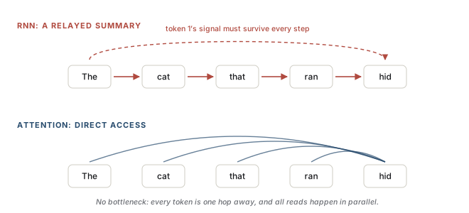
Before transformers, sequence models processed tokens one at a time, carrying a running summary in a hidden state (RNNs, LSTMs (Hochreiter & Schmidhuber, 1997)). Two problems followed: information from far back got squeezed through a bottleneck and faded, and the sequential dependency made training hard to parallelize.
Attention removes the bottleneck. Instead of forcing everything through a single evolving state, it lets each token reach back and read directly from any earlier token, with the strength of each read learned from context — an idea that first appeared as a bolt-on to translation RNNs (Bahdanau et al., 2015) before the transformer made it the whole machine.
Analogy
Reading a mystery novel, you hit the word "she" and instantly glance back to whichever earlier name it refers to — maybe twenty pages ago, maybe one sentence. You are not replaying every page; you jump straight to the relevant spot. Attention is that glance, computed for every word at once. It leaks in that the model has no true memory across separate calls — each glance only reaches within the current context window.
4.2Queries, keys, and values
Each token's vector is projected into three roles. For a token embedding \(x_i\):
- a query \(q_i = x_i W_Q\) — what this token is looking for,
- a key \(k_j = x_j W_K\) — what token \(j\) advertises about itself,
- a value \(v_j = x_j W_V\) — what token \(j\) will hand over if attended to.
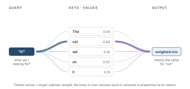
Token \(i\) scores every token \(j\) by the dot product \(q_i \cdot k_j\): high when the query and key point the same way. Those scores become weights via softmax, and the output for token \(i\) is the weighted sum of values.
Analogy
It is a soft dictionary lookup. The query is your search term, each key is an entry's label, and the value is its content. A hard dictionary returns the one exact match; attention returns a blend of all entries, weighted by how well each label matches — a lookup with no misses, only degrees of relevance.
Stacked over the whole sequence, this is a few matrix multiplies:
The \(QK^\top\) term is an \(n \times n\) matrix of every-token-against-every-token scores — which is exactly why cost grows with the square of sequence length, the fact behind every long-context headache in Chapter 15. In practice the wall is often memory movement, not raw arithmetic: FlashAttention computes the exact same softmax tile by tile without ever materializing that \(n \times n\) matrix, and at inference the per-token keys and values are cached rather than recomputed — both deferred to Chapter 15.
Interview
Why divide by \(\sqrt{d_k}\)? For large head dimension \(d_k\), dot products have variance that grows with \(d_k\), pushing softmax into saturated regions where gradients vanish. Scaling by \(\sqrt{d_k}\) keeps the scores' variance near 1 so the softmax stays in a responsive range. Forgetting this term is a classic cause of training instability.
4.3Multiple heads
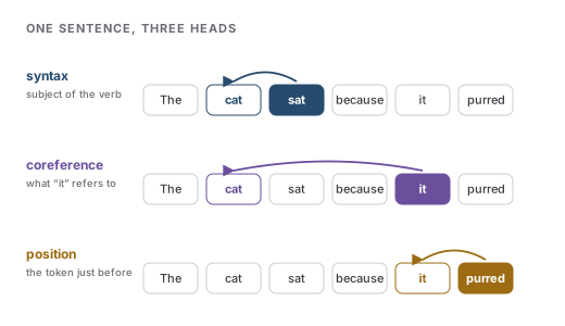
One attention operation blends everything into a single relevance signal. That is limiting: the relationship a pronoun has to its antecedent is not the relationship a verb has to its subject. Multi-head attention runs several attention operations in parallel, each with its own \(W_Q, W_K, W_V\) in a lower-dimensional subspace, then concatenates their outputs and projects back.
Intuition
Heads are specialists reading the same sentence for different things: one tracks syntax, another coreference, another position. You give the model several narrow lookups instead of one muddy one, then let it combine their findings.
If the model dimension is \(d\) and you use \(h\) heads, each head works in dimension \(d/h\), so multi-head attention costs about the same as single-head — you are partitioning the budget, not enlarging it.
4.4Causal masking
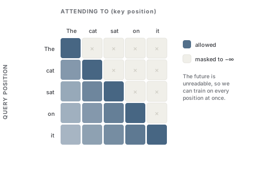
An LLM must predict the next token from past tokens only; letting position \(i\) attend to position \(i+1\) during training would leak the answer. The fix is a causal mask: before the softmax, set every score for a future position to \(-\infty\) so it receives zero weight.
Common trap
Break the mask and your eval loss looks magically low while the model has secretly been reading ahead. A loss that is suspiciously good early in training is the classic symptom.
Because the mask guarantees each position sees only earlier ones, every position can be trained at once against the real next token — conditioning on the ground-truth prefix, which is called teacher forcing. That is also where the train/generate asymmetry comes from: training is parallel over a known sequence, but generation has no ground truth, so the model must feed on its own samples one step at a time.
Interview
When would you reach for an encoder (BERT-style) instead of a decoder? When the whole input is available and you need to understand it rather than continue it — classification, retrieval embeddings, span extraction. An encoder attends bidirectionally and is trained with masked-language-modeling, so every token sees both sides (Devlin et al., 2019). A decoder is causal and autoregressive, built for generation. An encoder-decoder (T5-style) splits the two — a bidirectional encoder for the source, a causal decoder for the output — which suits translation and summarization (Raffel et al., 2020). The mistake is treating "transformer" as one thing; the attention pattern and objective are the real fork.
4.5The rest of the block
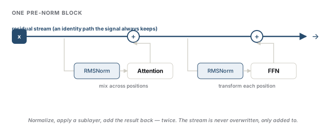
Attention moves information between positions. A transformer block pairs it with a feed-forward network (FFN) that processes each position independently, plus the connective tissue that makes deep stacks trainable:
# One pre-norm transformer block (schematic, not optimized).
def block(x):
    x = x + attention(rms_norm(x))       # Mix information across positions.
    x = x + feed_forward(rms_norm(x))    # Transform each position on its own.
    return x
Three pieces are doing quiet but essential work:
- Residual connections (the
x + ...) give gradients a clean path around each sublayer, so stacking 80 blocks does not kill training (He et al., 2016). Think of them as an express lane the signal can always take. - Normalization keeps activations in a stable range. Modern models normalize before each sublayer (pre-norm) rather than after, which trains more stably at depth (Xiong et al., 2020); Chapter 5 covers why RMSNorm replaced LayerNorm.
- The FFN is usually two linear layers with a nonlinearity, widening to roughly \(4d\) and back. It is where most of the parameters — and, many argue, most of the stored knowledge — live. Attention decides what to look at; the FFN decides what to make of it.
Interview
Where are a transformer's parameters? Roughly two-thirds sit in the FFNs and one-third in the attention projections (for typical shapes). This is why mixture-of-experts models (Chapter 5) target the FFN when they want to add capacity cheaply — they swap the single FFN for many, activating only a few per token.
4.6The full stack
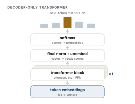
A decoder-only transformer is then just:
- Embed each token id into a vector, and add positional information (Chapter 5 explains why modern models use rotary embeddings instead of the original sinusoids).
- Repeat the block \(L\) times — 32 for a small model, 80-plus for a large one.
- Un-embed: a final linear layer maps the last position's vector to a score for every vocabulary token, and softmax turns those into the next-token distribution. Many models tie this layer to the input embedding — one shared matrix for both directions — saving a vocabulary-by-dimension block of parameters.
Intuition
The whole network is a tall stack of the same move: mix across positions with attention, then refine each position with an FFN, over and over. Depth lets early layers handle surface patterns and later layers assemble them into meaning.
That is the architecture every chapter after this one takes for granted. Chapter 5 shows how today's models tweak each component — positions, normalization, activations, and attention itself — for stability and efficiency at scale.
References
- Bahdanau, D., Cho, K., & Bengio, Y. (2015). Neural machine translation by jointly learning to align and translate. International Conference on Learning Representations. arXiv:1409.0473.
- Devlin, J., Chang, M.-W., Lee, K., & Toutanova, K. (2019). BERT: Pre-training of deep bidirectional transformers for language understanding. North American Chapter of the Association for Computational Linguistics. arXiv:1810.04805.
- He, K., Zhang, X., Ren, S., & Sun, J. (2016). Deep residual learning for image recognition. IEEE Conference on Computer Vision and Pattern Recognition. arXiv:1512.03385.
- Hochreiter, S., & Schmidhuber, J. (1997). Long short-term memory. Neural Computation, 9(8).
- Raffel, C., Shazeer, N., Roberts, A., Lee, K., et al. (2020). Exploring the limits of transfer learning with a unified text-to-text transformer. Journal of Machine Learning Research, 21(140). arXiv:1910.10683.
- Vaswani, A., Shazeer, N., Parmar, N., Uszkoreit, J., Jones, L., Gomez, A. N., Kaiser, Ł., & Polosukhin, I. (2017). Attention is all you need. Advances in Neural Information Processing Systems. arXiv:1706.03762.
- Xiong, R., Yang, Y., He, D., Zheng, K., Zheng, S., Xing, C., Zhang, H., Lan, Y., Wang, L., & Liu, T.-Y. (2020). On layer normalization in the transformer architecture. International Conference on Machine Learning. arXiv:2002.04745.
Check yourself
Interview-style questions on this chapter. Pick an answer to see whether it holds up.
-
You need high-quality sentence embeddings for retrieval and classification over inputs that are always fully available. Why might a BERT-style encoder beat a decoder-only LLM here?
The families differ by attention and objective: encoders (BERT-style, bidirectional MLM) see both directions and excel at encoding a fixed input; decoders (GPT-style, causal) are made for generation; encoder-decoder models (T5-style) split the two for sequence-to-sequence. Matching the architecture to 'understand a whole input' versus 'generate a continuation' is the point. -
Why is dividing the attention scores by the square root of the head dimension important?
Query-key dot products sum over the head dimension, so their variance grows with it. Without the square-root scaling, large scores saturate the softmax, gradients vanish, and training destabilizes. It is a classic source of instability when omitted. -
The causal mask lets a transformer train on every position of a sequence at once. What is the name for conditioning each prediction on the ground-truth previous tokens, and what asymmetry does it create?
Because the mask guarantees each position only sees earlier ones, every position can be trained simultaneously against the real next token (teacher forcing). At generation time there is no ground truth, so the model feeds on its own outputs sequentially, the source of the train/generate asymmetry (and of exposure bias). -
Roughly where do a transformer's parameters live, and why does it matter for mixture-of-experts models?
For typical shapes the FFNs hold about two-thirds of the parameters and, many argue, most of the stored knowledge. That is exactly why MoE targets the FFN: replace one FFN with many experts, route each token to a couple, and total capacity grows while per-token compute stays roughly fixed. -
A candidate claims the O(n^2) cost of attention means long-context models are fundamentally limited by compute. What is the more precise picture?
The n-by-n score matrix drives the quadratic compute, but the practical wall is often reading and writing that matrix to memory. FlashAttention reorders the computation to keep tiles in fast on-chip memory and never stores the full matrix, cutting memory traffic without changing the math. The serving-side consequences are Chapter 15's subject.