7Training Dynamics at Scale

A pretraining run is Chapter 2's five-line loop with the safety rails removed: one pass over trillions of tokens, on thousands of GPUs, for weeks or months, with no chance to start over if week six goes wrong. You cannot grid-search a run you can only afford once. What replaces the grid search is a small set of scaling rules, a trained eye for the loss curve, and machinery for keeping a long run alive. That is this chapter: the knobs you set before launch, the signals you watch after it, and what you do when the signals go bad.

7.1Batch size, learning rate, and warmup

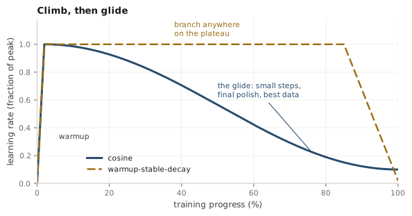
Every large run uses the same learning-rate shape: climb, then glide. Warmup ramps the learning rate linearly from zero over the first fraction of a percent of training; decay — usually a cosine — then lowers it smoothly to a small fraction of its peak by the final token (Loshchilov & Hutter, 2017). Warmup exists because the start of training is the most dangerous part: the weights are random, the first gradients are huge and unrepresentative, and Adam's per-parameter gradient statistics (Chapter 2) are estimated from almost no samples. Large steps taken on garbage statistics can wreck the run in its first thousand steps; warmup keeps steps tiny until the optimizer's bookkeeping is trustworthy. The decay end matters just as much — the final low-learning-rate stretch is where the loss quietly earns its last few percent, which is exactly why Chapter 6's data annealing is timed to it.

Batch size is the other pre-launch commitment, and it obeys a diminishing-returns law. Averaging more examples per step reduces gradient noise, so bigger batches support proportionally bigger learning rates — the linear scaling rule (Goyal et al., 2017). But once the batch is large enough that noise no longer dominates, doubling it again buys almost nothing: the gradient is already accurate, and you are spending twice the compute per step to take essentially the same step. The crossover point — the critical batch size — can be estimated from the gradient's own noise statistics, and it grows as the loss falls, which is why large runs often increase batch size mid-training (McCandlish et al., 2018).

7.2Loss curves and what they tell you

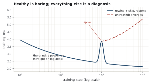
The training loss is the run's vital sign, and healthy is boring: a fast early drop as the model learns token frequencies and grammar, then an ever-slower grind that looks like a straight line on a log-scale plot — the power law Chapter 9 makes precise. Deviations from boring are diagnoses:

• A plateau that arrives too early usually means the learning rate is too low, the data loader is recycling (the model has seen this before), or a preprocessing bug is feeding degenerate batches.
• A spike — the loss jumps sharply and then may or may not recover — is the signature event of large-scale training. PaLM's team reported roughly twenty of them across a run, each at a scale where the same data replayed from a different checkpoint caused no spike: the trigger is a bad collision of model state and batch, not a bad batch alone (Chowdhery et al., 2023).
• Divergence — the loss climbs and keeps climbing — means the run is dead and something structural was wrong: learning rate too high, a precision problem (Chapter 2's fp16 range trap), or missing normalization.

The standard spike response is unglamorous: rewind to the last good checkpoint, skip a few hundred batches, resume (Chowdhery et al., 2023). Prevention is the next section's subject.

7.3Stability tricks

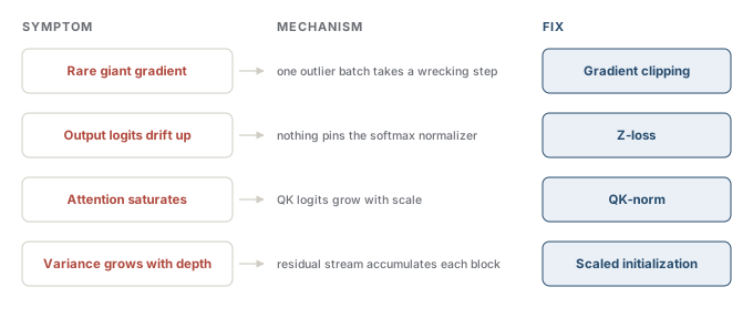
Each stability trick in the modern recipe is a patch over a specific, named failure. Four cover most of what you will meet:

• Gradient clipping rescales any batch gradient whose global norm exceeds a threshold (typically 1.0). It converts a rare catastrophic step into a merely wasted one — a shock absorber, not a steering input. If clipping fires often, the learning rate is wrong; the trick is for outliers.
• Z-loss addresses a slow drift in the final softmax: nothing in cross-entropy prevents the logits from all growing together, and in low precision that growth eventually misbehaves. Z-loss adds a small penalty on the softmax normalizer, pinning the logit scale (Chowdhery et al., 2023; Zoph et al., 2022).
• QK-norm normalizes queries and keys before their dot product, capping attention logits — the fix for attention-entropy collapse at scale, met already in Chapter 5 (Dehghani et al., 2023).
• Careful initialization and bf16 (Chapter 2) round out the kit: residual-branch scaling keeps the residual stream's variance flat with depth, and bf16's full exponent range removes the overflow failure fp16 invited.

7.4Checkpointing and reproducibility

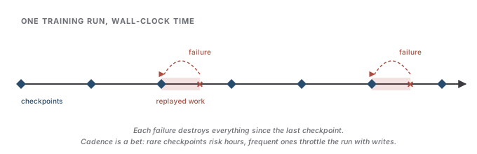
At cluster scale, hardware failure is not a risk; it is a schedule. Chain thousands of GPUs into one synchronous computation and the run's time-between-failures shrinks to hours — Llama 3's team logged over four hundred unexpected interruptions across a 54-day run, the majority from GPU and memory faults (Grattafiori et al., 2024); the OPT team's public logbook records the same life at 175B scale, restart by restart (Zhang et al., 2022). The design consequence: a run is not a process that finishes but a process that resumes, and the checkpoint is its unit of survival.

A resumable checkpoint holds more than weights: the optimizer state (Adam's moments — twice the size of the model, per Chapter 8's accounting), the learning-rate schedule position, the data loader's exact position, and the random-number-generator states. Miss the data-loader state and resumption silently double-feeds part of the corpus — a bug that shows up in nothing but a slightly wrong model. Checkpoint frequency is its own small optimization: too rare and each failure burns hours of GPU-time; too frequent and the writes themselves throttle the run, which is why large jobs stage checkpoints asynchronously to fast local storage before shipping them off-node.

Exact reproducibility, meanwhile, is quietly abandoned at scale, for a reason worth knowing precisely: floating-point addition is not associative — \((a+b)+c\) and \(a+(b+c)\) can differ in the last bit — and GPU kernels sum in whatever order the hardware schedules, which varies run to run. Those last-bit differences feed a chaotic system millions of times, so two "identical" runs part ways. What teams actually guarantee is statistical reproducibility — same data, same seeds, same curve shape — plus bitwise-faithful resumption from a checkpoint, which is a much narrower promise.

Everything here assumed the model already fits on the hardware and the steps already run fast. Making that true is its own discipline — the next chapter's subject.

References

- Chowdhery, A., Narang, S., Devlin, J., Bosma, M., et al. (2023). PaLM: Scaling language modeling with Pathways. Journal of Machine Learning Research, 24(240). arXiv:2204.02311.
- Dehghani, M., Djolonga, J., Mustafa, B., Padlewski, P., et al. (2023). Scaling vision transformers to 22 billion parameters. International Conference on Machine Learning. arXiv:2302.05442.
- Goyal, P., Dollár, P., Girshick, R., Noordhuis, P., et al. (2017). Accurate, large minibatch SGD: Training ImageNet in 1 hour. arXiv preprint. arXiv:1706.02677.
- Grattafiori, A., Dubey, A., Jauhri, A., Pandey, A., et al. (2024). The Llama 3 herd of models. arXiv preprint. arXiv:2407.21783.
- Hu, S., Tu, Y., Han, X., He, C., et al. (2024). MiniCPM: Unveiling the potential of small language models with scalable training strategies. arXiv preprint. arXiv:2404.06395.
- Loshchilov, I., & Hutter, F. (2017). SGDR: Stochastic gradient descent with warm restarts. International Conference on Learning Representations. arXiv:1608.03983.
- McCandlish, S., Kaplan, J., Amodei, D., & OpenAI Dota Team (2018). An empirical model of large-batch training. arXiv preprint. arXiv:1812.06162.
- Zhang, S., Roller, S., Goyal, N., Artetxe, M., et al. (2022). OPT: Open pre-trained transformer language models. arXiv preprint. arXiv:2205.01068.
- Zoph, B., Bello, I., Kumar, S., Du, N., et al. (2022). ST-MoE: Designing stable and transferable sparse expert models. arXiv preprint. arXiv:2202.08906.
Check yourself
Interview-style questions on this chapter. Pick an answer to see whether it holds up.
-
Why does every large training run begin with learning-rate warmup rather than starting at the peak rate?
Adam divides each update by a running estimate of gradient magnitude; with a handful of samples that denominator is noise, so effective step sizes are erratic exactly when gradients are largest. Warmup is insurance against those first few thousand steps. Its length is measured in steps, not epochs - typically a fraction of a percent of the run. -
What does the critical batch size mark, and what happens if you train beyond it?
McCandlish et al. (2018) estimate it from the gradient noise scale: while noise dominates, bigger batches let you take proportionally bigger steps (the linear scaling rule); once the gradient estimate is already accurate, more averaging is waste. Since the noise scale grows as the loss falls, large runs often ramp the batch size up during training. -
During a large run the loss spikes sharply. The team rewinds to a checkpoint and skips a few hundred batches. Replaying the same batches from a different checkpoint causes no spike. What does this reveal about spikes?
PaLM's team documented exactly this: the same data replayed from a different state trained fine, implying the state-times-batch interaction, not the batch, is the trigger. This is also why spike prevention is about damping mechanisms (clipping, z-loss, QK-norm) rather than data cleaning. -
What problem does z-loss solve in large-scale training?
The softmax output depends only on logit differences, so the absolute scale is a free parameter that can drift over a long run - harmless in fp32, dangerous in bf16. Z-loss (PaLM, ST-MoE) adds a small penalty on log-sum-exp of the logits, anchoring the scale. It is a stability patch, not a regularizer for generalization. -
Two launches of the same training job - same code, same data, same seeds - produce measurably different weights. What is the root cause?
Parallel reductions schedule their partial sums differently run to run, and (a+b)+c differs from a+(b+c) in floats. Each difference is one ulp, but training dynamics amplify rather than damp them. Teams therefore promise statistical reproducibility and bitwise-faithful checkpoint resumption, not bit-identical end-to-end runs.