19Asymptotic Efficiency

Maximum likelihood (Chapter 8) was sold to you on a promise: pick the parameter that makes your data least surprising, and you get a general-purpose estimator that works across models. This chapter cashes the promise. It says why the maximum likelihood estimate deserves to be the default — not because it is unbiased or simple, but because, once you have enough data, its sampling distribution (Chapter 6) is the narrowest Gaussian the problem physically allows. The Cramér–Rao bound (Chapter 7) told you there is a floor on how tightly any estimator can concentrate; the large-sample theory of the maximum likelihood estimate tells you that estimator walks right up to that floor and stands on it, and — the deeper and more surprising claim — that essentially nothing can do better.

If you take one idea from this chapter, take this: with enough data the maximum likelihood estimate becomes Gaussian, centered on the truth, with a variance equal to the inverse Fisher information — the smallest variance any well-behaved estimator can have — so "efficient" stops being a property you check and becomes the standard everything else is measured against.

19.1Large-sample behavior of the MLE

Two facts, stacked, carry this whole section. The first is consistency: as the sample size \(n\) grows, the maximum likelihood estimate \(\hat\theta_n\) converges in probability (Chapter 5) to the true parameter \(\theta_0\). Feed the estimator more data and it homes in on the right answer; the sampling distribution collapses toward a spike at the truth. The intuition is that the log-likelihood, averaged over the sample, converges by the law of large numbers (Chapter 5) to a fixed curve whose unique peak sits at \(\theta_0\) — so the sample's peak, which is \(\hat\theta_n\), has nowhere to go but the truth. This is not automatic: it needs the model to be identifiable (different parameters must give genuinely different distributions, or the peak is not unique) and correctly specified, among other conditions we return to below.

Consistency alone is weak — it says you arrive, not how fast or with what spread. The second fact supplies both. Under the regularity conditions, the maximum likelihood estimate is asymptotically normal (its rescaled sampling distribution approaches a Gaussian):

where \(I(\theta_0)\) is the Fisher information (Chapter 7), the curvature of the log-likelihood — how sharply the data, on average, distinguishes \(\theta_0\) from its neighbors. Undo the \(\sqrt{n}\) scaling and the practical reading is that for large \(n\) the sampling distribution of the estimate itself is approximately

The variance shrinks like \(1/n\), so the standard error shrinks like \(1/\sqrt{n}\) — the same rate the central limit theorem (Chapter 5) sets for a sample mean, and no accident, because the derivation is a central limit theorem in disguise. Here is the mechanism in one breath. The estimate solves the score equation — it sets the derivative of the log-likelihood, the score, to zero (Chapter 7). The score is a sum of independent per-observation terms with mean zero and variance \(I(\theta_0)\), so by the central limit theorem it is asymptotically Gaussian; a one-step Taylor expansion of the score around \(\theta_0\) then divides that Gaussian numerator by the log-likelihood's curvature, which converges to \(I(\theta_0)\). Gaussian on top, information on the bottom: out falls \(\mathrm{Normal}(0, I^{-1})\).

Because \(I(\theta_0)^{-1}/n\) is exactly the Cramér–Rao floor for an unbiased estimator (Chapter 7), an estimator whose asymptotic variance equals \(I(\theta_0)^{-1}\) is called asymptotically efficient — it achieves the information bound in the limit, wasting none of the data's discriminating power. The maximum likelihood estimate is the canonical example. This is the sense in which it is not merely a good estimator but the yardstick: any competitor is graded by how close its asymptotic variance comes to the same floor.

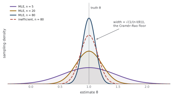
The word asymptotic is doing real work, and the regularity conditions are where honest treatments earn their keep. The clean Gaussian limit needs several things at once: the model must be correctly specified and identifiable; the log-likelihood must be smooth enough to differentiate twice; the Fisher information must be finite and nonzero; the true parameter must lie in the interior of the parameter space, not on a boundary; and the support of the distribution must not depend on the parameter. Break any of these and the story changes. When \(\theta_0\) sits on a boundary — a variance component pinned at zero — the limit is no longer a clean Gaussian but a truncated or mixture law (the same boundary problem that bent Wilks' theorem in Chapter 16). When the support depends on \(\theta\), as for the uniform distribution on \([0,\theta]\) whose likelihood peaks at a corner rather than a smooth interior maximum, the estimate converges at rate \(1/n\) rather than \(1/\sqrt{n}\) and its limit is exponential, not Gaussian — faster than "efficient," but outside the theory entirely. And when identifiability fails, consistency itself collapses because the likelihood has no unique peak to find.

19.2The information floor, again

The Cramér–Rao bound arrived in Chapter 7 as a finite-sample fact with a catch: it lower-bounds the variance only of unbiased estimators. Since the maximum likelihood estimate is usually biased, that bound does not literally apply to it — yet its asymptotic variance lands exactly on the floor. The asymptotic theory is what resolves the tension, and it does more than the finite-sample bound could: it says the floor is optimal not just among unbiased estimators but among essentially all reasonable ones. Making that precise is the achievement of the local asymptotic framework, and it is worth stating honestly rather than waving at, because it is the rigorous backbone under the loose slogan "you cannot beat the MLE."

The framework's engine is local asymptotic normality (LAN): near the truth, on the \(1/\sqrt{n}\) scale where the estimate actually lives, the whole statistical model starts to look like one clean idealized problem — estimating the mean of a single Gaussian with known variance \(I(\theta_0)^{-1}\). Formally, the log-likelihood ratio between \(\theta_0 + h/\sqrt{n}\) and \(\theta_0\) expands into a quadratic in the local parameter \(h\), the signature of a Gaussian-shift experiment (Le Cam, 1953; van der Vaart, 1998). Le Cam's insight is that once your model is LAN, every question about efficient estimation transfers to that limiting Gaussian problem — where the answer is known and simple — so you never have to fight the original model's idiosyncrasies. This is the machinery, developed by Le Cam and Hájek, that upgrades "the MLE happens to hit the floor" into "the floor is a wall no one can pass."

Two theorems build the wall. The first is the convolution theorem (Hájek, 1970). Restrict attention to regular estimators — those whose limiting behavior does not lurch discontinuously as the true parameter is nudged locally, a mild condition ruling out pathological rules that exploit one exact parameter value. Hájek's theorem says the limiting distribution of any regular estimator is a convolution: the efficient Gaussian \(\mathrm{Normal}(0, I^{-1})\) plus independent extra noise. You can add junk on top of the efficient distribution, but you can never subtract from it — the best achievable limit is the pure Gaussian with no added noise, which is exactly what the maximum likelihood estimate attains. The second is the local asymptotic minimax (LAM) theorem (Hájek, 1972; Le Cam, 1953): for any sensible ("bowl-shaped") loss, no estimator can beat the risk of the efficient Gaussian in the worst case over a shrinking neighborhood of the truth. Where the convolution theorem constrains regular estimators, LAM drops even that restriction and bounds every estimator, at the cost of judging it by its worst nearby parameter rather than a single point.

That cautionary tale is superefficiency: the existence of estimators that beat the information bound — smaller asymptotic variance than \(I^{-1}\) — at some parameter values. The famous construction is Hodges' estimator (Le Cam, 1953). Start from the maximum likelihood estimate \(\hat\theta\), and add one rule: if \(\hat\theta\) falls within \(n^{-1/4}\) of zero, snap it to exactly \(0\); otherwise leave it alone. When the truth really is \(\theta_0 = 0\), this shrink-to-zero move makes the estimator ferociously accurate — asymptotic variance \(0\), cleanly below the floor \(I^{-1}\). For a while in the 1950s this looked like it might break the whole efficiency story: an estimator that beats the "unbeatable" bound.

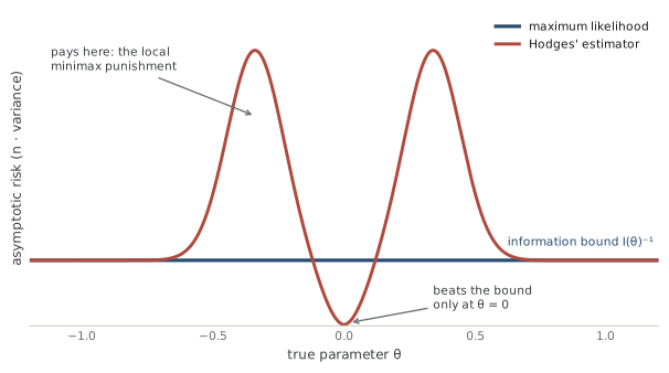
It does not break it, and seeing why is the point of the whole framework. Two facts defang Hodges' estimator. First, the set of parameter values where any estimator can be superefficient has Lebesgue measure zero — Le Cam proved you can win at isolated points but never on a region of real width, so the "improvement" is invisible to any prior that spreads mass continuously. Second, and this is what LAM is for: buying that dip at \(\theta_0 = 0\) costs you enormously in a neighborhood around zero, where the estimator's risk spikes far above the floor (the peaks in the figure). Because LAM judges an estimator by its worst case over a shrinking neighborhood — not by its value at one lucky point — it sees those peaks, and the maximum likelihood estimate, flat on the floor everywhere, wins the local-minimax contest. Superefficiency at a point is real; superefficiency that survives the honest worst-case accounting does not exist.

When two estimators both work, you compare them by relative efficiency — the ratio of their asymptotic variances (equivalently, the ratio of sample sizes each needs to reach the same precision). An estimator with relative efficiency \(0.8\) against the maximum likelihood estimate needs about \(25\%\) more data to match it, because it wastes a fifth of the information. Since the maximum likelihood estimate sits on the floor, its relative efficiency against any competitor is at least \(1\): efficiency is the currency in which "how much does using the wrong method cost?" gets a number.

All of this, though, rests on a foundation stated once and then quietly assumed everywhere: the model is correct. Drop that and the picture shifts. Cast the maximum likelihood estimate as an M-estimator — an estimator defined as the solution to an estimating equation, "set the average of some score function to zero" — and you can ask what it converges to when the data does not come from your assumed family. Under misspecification (the model family does not contain the true data-generating distribution), the estimate still converges and is still asymptotically normal, but it aims at the parameter value whose model is closest to the truth in Kullback–Leibler divergence, and its asymptotic variance is no longer the tidy \(I^{-1}\). Instead it takes the sandwich form (White, 1982):

The name is the shape: two "bread" factors \(A^{-1}\) around a "meat" factor \(B\). When the model is correct, a beautiful identity from Chapter 7 — the two definitions of Fisher information agree — forces \(A = B = I\), the bread and meat cancel, and the sandwich collapses to the efficient \(I^{-1}\). When the model is wrong, \(A \neq B\), the collapse fails, and reporting the naive \(I^{-1}\) standard error understates (or overstates) the real uncertainty. The efficiency guarantee is a reward for a correctly specified model; the sandwich is what you fall back on when you are honest that yours might not be.

References

- Hájek, J. (1970). A characterization of limiting distributions of regular estimates. Zeitschrift für Wahrscheinlichkeitstheorie und verwandte Gebiete.
- Hájek, J. (1972). Local asymptotic minimax and admissibility in estimation. Proceedings of the Sixth Berkeley Symposium on Mathematical Statistics and Probability.
- Le Cam, L. (1953). On some asymptotic properties of maximum likelihood estimates and related Bayes' estimates. University of California Publications in Statistics.
- van der Vaart, A. W. (1998). Asymptotic Statistics. Cambridge University Press.
- White, H. (1982). Maximum likelihood estimation of misspecified models. Econometrica.
Check yourself
A few questions to test the ideas from this chapter. Pick an answer to see whether it holds up.
-
Under the usual regularity conditions, what does asymptotic normality of the MLE assert about √n(θ̂ − θ₀)?
The √n rescaling is exactly what stops the variance collapsing to zero — that collapse is consistency, the separate and weaker fact that θ̂ itself converges to θ₀. The information enters inverted because curvature and uncertainty are reciprocals: a sharply peaked likelihood (large I) pins the parameter down (small variance). -
The MLE for the Uniform(0, θ) model converges at rate 1/n to a non-Gaussian limit, outside the standard theory. Which regularity condition does this model break?
The score-equation derivation of asymptotic normality needs a smooth interior maximum. When the support edge moves with θ the maximizer is max xᵢ — a corner, not a stationary point — and the estimate actually converges faster than √n (rate 1/n), with an exponential limit. Identifiability holds here, and the pathology is the moving support, not the information. -
Hájek's convolution theorem characterizes the limiting distribution of any regular estimator. What does it say?
Convolving with independent noise can only spread a distribution, never sharpen it, so I⁻¹ is a floor — but the theorem does not force equality: inefficient regular estimators exist, carrying extra noise. The restriction to 'regular' estimators is the escape hatch superefficient rules exploit, and the whole point of the asymptotic theory is that it transcends the unbiased-only restriction of the finite-sample Cramér–Rao bound. -
Hodges' estimator has asymptotic variance strictly below I⁻¹ at θ = 0. Why does this not make the MLE asymptotically inadmissible?
Inadmissibility requires domination: no worse everywhere and strictly better somewhere. Hodges wins only on a measure-zero set and loses badly in the surrounding neighborhood (the local-minimax risk peaks), so it does not dominate. Contrast the James–Stein estimator (Chapter 13), which genuinely dominates the sample mean everywhere in three or more dimensions — a real free lunch, where Hodges is a fake one. -
You fit a model by maximum likelihood but suspect the model family does not contain the true distribution. What asymptotic variance should you report?
Under misspecification the two forms of the information identity — expected Hessian versus score variance — no longer coincide, so A ≠ B and the sandwich does not collapse to I⁻¹. The estimate also targets the parameter whose model is closest in Kullback–Leibler divergence, not the true distribution, so it is not consistent for the truth; reporting the naive I⁻¹ can badly misstate the real uncertainty. -
An estimator has asymptotic relative efficiency 0.5 against the MLE. What does that mean operationally?
Relative efficiency is the ratio of asymptotic variances; 0.5 means twice the variance, and since variance scales like 1/n, matching the MLE's precision takes about twice the sample size. It does not change the √n convergence rate, and a value below 1 always means worse (larger variance), never beating the floor.