17P-values, Power, and Errors
Hypothesis testing, Chapter 16, gave you the machinery: a null hypothesis, a test statistic, and a rejection rule calibrated to a false-positive rate. This chapter is about the number that machinery spits out and the number you should have computed before you ever collected data. The first is the p-value, the most used and most misread quantity in all of statistics. The second is power, the quantity a careful analyst pins down first and a careless one never computes at all. Getting these two straight is most of what separates a result that replicates from one that evaporates.
If you take one idea from this chapter, take this: a p-value measures surprise under the null, not the probability that the null is false — and a study too small to detect the effect it is hunting will lie to you in both directions at once.
17.1What a p-value is and is not
Start with the definition, stated precisely, because almost every misuse is a slide away from it. Fix a null hypothesis \(H_0\) and a test statistic \(T\) whose large values count as evidence against \(H_0\). You collect data and observe the value \(t_{\text{obs}}\). The p-value is the probability, computed assuming \(H_0\) is true, of drawing a test statistic at least as extreme as the one you saw:
Read it slowly. Everything to the right of the bar is a hypothesis, not a fact; the probability lives in the sampling distribution of \(T\) under \(H_0\), not in the world. The p-value answers one narrow question — if the null were true, how often would chance alone hand me data this contrary to it? — and a small answer means your data sit far out in the tail the null predicts.
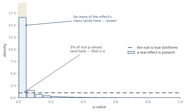
That is the whole honest content of the number, and it comes with a clean structural fact. If \(H_0\) is true and \(T\) is continuous, the p-value is Uniform on \([0,1]\): every value between 0 and 1 is equally likely. A p-value below 0.05 is no rarer than one between 0.90 and 0.95 when the null holds; each has probability 0.05. This uniformity is what makes the whole apparatus honest, because it is exactly what guarantees that testing at level \(\alpha\) rejects a true null a fraction \(\alpha\) of the time — the Type I error rate (the probability of rejecting a true null, Chapter 16) you chose.
A sharper question
If the null is true, why is the p-value exactly Uniform rather than just "usually large"? Because the p-value is the null's own tail probability applied to a draw from the null. Write \(F\) for the CDF of \(T\) under \(H_0\); the p-value is essentially \(1 - F(T)\), and plugging a random variable into its own CDF is the probability integral transform, which returns a Uniform\((0,1)\) (random variables and their distributions, Chapter 1). The uniformity is not a convenient approximation — it is the load-bearing fact that lets you set a false-positive rate at all. It leaks only when \(T\) is discrete (counts, exact tests), where the p-value can be Uniform-ish but lumpy, making the achievable \(\alpha\) come in steps rather than a continuum.
Now the misreadings, because the definition is narrow and the temptations are wide. Each of the traps below is a well-worn path, and each has been walked into print thousands of times.
Common trap
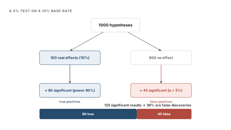
A p-value is not the probability that the null hypothesis is true. That quantity, \(\Pr(H_0 \mid \text{data})\), is a posterior probability and requires a prior (the Bayesian view, Chapter 9); the p-value deliberately conditions the other way, on \(H_0\) rather than on the data. Confusing \(\Pr(\text{data} \mid H_0)\) with \(\Pr(H_0 \mid \text{data})\) is the prosecutor's fallacy: "the DNA match is rare if he is innocent" is not "he is probably guilty," and the gap between them is exactly the base rate the next figure makes concrete.
Common trap
A p-value is not an effect size and says nothing about whether an effect matters. It blends the size of the effect with the size of the study: pour in enough data and a trivially small, practically meaningless difference will eventually cross any threshold, while a large, important effect measured on a handful of subjects may not. "Statistically significant" means "distinguishable from the null given this sample size," which is a claim about detectability, not about magnitude or importance. Report the estimate and its interval (Chapter 18); the p-value alone hides the thing you actually care about.
Common trap
A p-value is not the probability that the result will replicate, and \(1 - p\) is not your confidence in the finding. A single p-value carries no information about the next experiment's outcome; a study can produce \(p = 0.01\) and have a coin's chance of reaching significance again, because replication probability depends on the true effect and the new study's power, neither of which the p-value contains.
These are not fringe errors, which is why the American Statistical Association took the unusual step of issuing a formal statement on them (Wasserstein & Lazar, 2016). Its principles are worth carrying: p-values can indicate incompatibility between data and a model, but they do not measure the probability that the hypothesis is true or that the data arose by chance alone; scientific conclusions should not rest on whether a p-value crosses a threshold; and a p-value reported without the effect size, the design, and the full analysis is close to meaningless.
The deepest trap is thinking a small p-value means a likely-true finding, and defusing it needs the base rate — the fraction of hypotheses you test that correspond to real effects (Chapter 9). Suppose you screen 1000 hypotheses of which only 10% are real, you test each at \(\alpha = 0.05\), and your power is 80%. The 100 real effects yield about 80 true discoveries; the 900 nulls yield about \(0.05 \times 900 = 45\) false ones. Of the 125 results you call significant, 45 — better than one in three — are false, even though every single one cleared \(p < 0.05\). The fraction of your "discoveries" that are wrong is the false discovery rate (FDR), and when the base rate of real effects is low, a nominal 5% test can run an FDR north of 30%. This is the arithmetic behind the claim that most published findings in some fields are false (Ioannidis, 2005): low base rates, modest power, and flexible analysis conspire so that "significant" is a weak signal of "true."
Intuition
A small p-value is a surprising card, not a verdict. It tells you the data would be unusual if nothing were going on — but whether something is going on also depends on how often something is going on in the pool you drew from. Rare-under-the-null and probably-real are the same only when real effects were plentiful to begin with; when they are scarce, the tide of true nulls throwing off the occasional false positive can outnumber the genuine hits.
A sharper question
Does a p-value of 0.049 and one of 0.051 differ in kind, given that one is "significant" and one is not? No — they are essentially the same evidence, and treating them as categorically different is the single most damaging habit the threshold encourages. The p-value is continuous, and 0.049 versus 0.051 is a hair's difference in tail probability; the 0.05 line is a convention Fisher floated, not a law of nature. Bucketing results into "significant" and "not" discards the continuity and invites the dichotomization the ASA warns against — the sense that crossing 0.05 flips a finding from false to true. The honest report is the number itself, with its interval and effect size, not which side of an arbitrary fence it landed on.
17.2Power and sample size
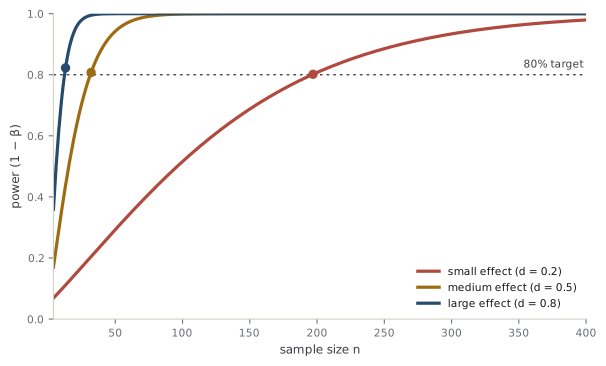
The p-value is computed after the data arrive; power is the question you must answer before. Power is the probability that your test rejects the null when a real effect of a given size is present — formally \(1 - \beta\), where \(\beta\) is the Type II error rate, the probability of missing a real effect (Chapter 16). A test with 80% power finds a true effect of the assumed size four times in five and misses it the fifth; at 50% power it is a coin flip whether a real effect ever shows up as significant. Asking "what is my power?" before collecting data is asking "if the effect I am hunting is really out there, do I even have a chance of catching it?" — and running a study without an answer is spending a research budget on a lottery ticket whose odds you declined to read.
Four levers set power, and you control some more than others. Power rises with the effect size — the true magnitude of what you are trying to detect, often measured in standard-deviation units so it is comparable across problems — because a bigger signal is easier to see. It rises as the noise variance falls, since less scatter means a cleaner view. It rises as you loosen \(\alpha\), because a more lenient rejection rule catches more of everything, true and false alike. And it rises with the sample size \(n\): more data shrinks the estimator's standard error like \(1/\sqrt{n}\) (the sampling distribution, Chapter 4), pulling the alternative's distribution away from the null until they barely overlap. Of the four, \(n\) is usually the only one you freely control, which is why "power analysis" in practice means solving for the sample size that buys a target power — commonly 80% — at a fixed \(\alpha\) and a planned-for effect size.
Intuition
Power is the resolving power of a microscope. A weak lens (small \(n\)) can still catch a large, obvious feature but will miss anything subtle; to see fine structure you need more magnification, and the finer the structure the more you need. Choosing a sample size is choosing how small an effect you are equipped to see — and if you point an underpowered instrument at a subtle effect, you are not being conservative, you are guaranteeing an uninterpretable result.
The cost of ignoring power is worse than merely missing effects, and this is the part that surprises people. An underpowered study does not just fail quietly; when it does reach significance, it systematically lies about the effect. The reason is a selection effect: at low power, only the luckiest, most inflated estimates clear the significance bar, so the significant ones are a biased sample of the truth — a winner's curse. Gelman and Carlin make this precise with two error types that survive even after you reject the null (Gelman & Carlin, 2014). A Type S error (sign) is getting the direction of the effect wrong — reporting a benefit that is really a harm. A Type M error (magnitude) is getting the size wrong — and in a low-power study the significant estimates can be inflated several-fold on average. So the underpowered study is doubly treacherous: it usually misses real effects, and on the occasions it "finds" one, the published number is exaggerated and sometimes pointed the wrong way.
A sharper question
If my study reached significance, why should I still worry about low power — didn't the significant result vindicate the design? No, and this is the winner's-curse trap in one question. Significance conditions on clearing the bar, and at low power only over-estimates clear it, so a "successful" underpowered study hands you an effect size that is biased upward by construction — the very selection that produced your \(p < 0.05\) also inflated your point estimate. Power is a property of the design, not of the outcome; a significant result from an underpowered study is more reason to distrust the magnitude, not less. This is why replication attempts, which are often better powered, so reliably find effects smaller than the original headline.
The problem compounds the moment you test more than one hypothesis, because every additional test is another chance for a null to slip through. Run 20 independent tests of true nulls at \(\alpha = 0.05\) and you expect one false positive; run a genomics screen of 20,000 and you expect a thousand. This is multiple testing, and there are two philosophies for taming it. The Bonferroni correction controls the family-wise error rate (FWER) — the probability of making even one false rejection across the whole family — by testing each of \(m\) hypotheses at level \(\alpha/m\). It is simple and airtight, but for large \(m\) it is brutally conservative: at \(\alpha/20000\) per test, all but the most violent effects are crushed along with the nulls, and power collapses. The Benjamini–Hochberg procedure controls the softer false discovery rate instead — the expected fraction of your rejections that are false — by sorting the \(m\) p-values \(p_{(1)} \leq \cdots \leq p_{(m)}\) and rejecting the largest run for which \(p_{(i)} \leq \frac{i}{m}\alpha\) (Benjamini & Hochberg, 1995). It tolerates a controlled sprinkle of false positives in exchange for far more discoveries, which is exactly the trade a screening study wants.
A sharper question
Why does controlling the false discovery rate beat Bonferroni for a large screen, if Bonferroni gives the stronger guarantee? Because the guarantees answer different questions, and for a screen the FDR question is the right one. Bonferroni promises "probably not a single false positive anywhere," a promise so strict that across 20,000 tests it sets the per-test bar so low it discards almost every real effect too — you buy near-zero false positives with near-zero discoveries. Benjamini–Hochberg promises instead "of the hundreds of hits I report, no more than 5% are false on average," which is what you actually care about when the output is a candidate list you will follow up anyway. It adapts to the data — the more small p-values there are, the more it rejects — so it recovers power that Bonferroni throws away, at the price of trading a never-any guarantee for an on-average one.
Note
The two error rates coincide when every null is true: with no real effects, any false positive is both "one false rejection" (FWER) and "100% of rejections false" (FDR), so controlling either controls the other. They diverge exactly when some effects are real — then FDR grants you the discoveries FWER would forbid. This is why Bonferroni is the right tool for a confirmatory test of a few pre-specified hypotheses, and Benjamini–Hochberg for an exploratory screen of thousands.
All of this feeds the replication crisis: the finding across psychology, medicine, and beyond that a large share of published, significant results do not hold up when someone repeats the study. The causes are now familiar — low power, low base rates, and analytic flexibility. That flexibility has a name, p-hacking: consciously or not, trying analyses until one crosses \(p < 0.05\) — dropping outliers, adding covariates, testing subgroups, peeking at the data and stopping when it looks good. Its subtler cousin is the garden of forking paths, where a researcher makes only one set of choices but those choices were contingent on the data, so a whole thicket of tests is implicitly run even though only one is reported. Both wreck the p-value's guarantee, because the Uniform-under-the-null property assumes a single, pre-specified test; search over many and you have quietly changed the null distribution. Add the file-drawer problem — significant results get published while null results sit in a drawer — and the literature itself becomes a biased sample of the experiments actually run.
Common trap
Pre-registration and a power analysis are not bureaucratic box-ticking; they are what restore the p-value's meaning. A p-value is only Uniform under the null if the test was fixed before the data spoke. The moment your stopping rule, your outcome, or your covariates depend on what you saw, you are somewhere in the garden of forking paths, and your reported 0.03 no longer means what its definition promises.
A sharper question
So should the field abandon statistical significance, or just make the threshold stricter? The discipline genuinely disagrees, and it is worth knowing the two camps. One proposes to redefine significance, lowering the default threshold for new discoveries from 0.05 to 0.005 so that a "significant" claim carries far stronger evidence (Benjamin et al., 2018). The other argues to retire the significant/not-significant dichotomy entirely — stop thresholding, report effect sizes and intervals, and treat evidence as continuous (Amrhein et al., 2019). They agree on the diagnosis, that mechanical thresholding drives the crisis; they differ on whether the cure is a better threshold or no threshold. The safe practical stance is the one both camps share: never let a single p-value carry a conclusion, always report the estimate and its uncertainty, and design for adequate power before you collect a thing.
References
- Amrhein, V., Greenland, S., McShane, B., et al. (2019). Scientists Rise Up Against Statistical Significance. Nature.
- Benjamin, D. J., et al. (2018). Redefine Statistical Significance. Nature Human Behaviour.
- Benjamini, Y., & Hochberg, Y. (1995). Controlling the False Discovery Rate: A Practical and Powerful Approach to Multiple Testing. Journal of the Royal Statistical Society, Series B.
- Gelman, A., & Carlin, J. (2014). Beyond Power Calculations: Assessing Type S (Sign) and Type M (Magnitude) Errors. Perspectives on Psychological Science.
- Ioannidis, J. P. A. (2005). Why Most Published Research Findings Are False. PLoS Medicine.
- Wasserstein, R. L., & Lazar, N. A. (2016). The ASA Statement on p-Values: Context, Process, and Purpose. The American Statistician.
Check yourself
A few questions to test the ideas from this chapter. Pick an answer to see whether it holds up.
-
A study reports p = 0.01. Which statement correctly describes what that number means?
A p-value is computed assuming the null holds; it is the tail probability of a test statistic at least as extreme as observed. It conditions on the null, so it is not the probability the null is true (that would need a prior and Bayes' rule). It is not a replication probability, which depends on the true effect and the new study's power, and it is not an effect size — a huge sample can make a trivial effect cross any threshold. -
Why is the p-value distributed Uniform(0,1) when the null hypothesis is true and the test statistic is continuous?
The p-value is essentially one minus the null CDF evaluated at the statistic, and feeding a variable through its own CDF is the probability integral transform, which returns a Uniform(0,1). This is exact for a continuous statistic, not an asymptotic approximation, and it is precisely what makes a level-α test reject a true null a fraction α of the time. With a discrete statistic the p-value is only lumpily uniform. -
You screen 1000 hypotheses at α = 0.05 with 80% power, and only 10% of the hypotheses correspond to real effects. Roughly what fraction of your significant results are false positives?
The 100 real effects yield about 80 true positives; the 900 nulls yield about 0.05 x 900 = 45 false positives. Of 125 significant results, 45 are false, roughly 36%. The significance level controls the error rate among nulls only; with a low base rate the sheer number of nulls dominates the mix, which is why a small p-value need not signal a likely-true finding. -
An underpowered study nonetheless reaches p < 0.05. Why should you distrust its reported effect size more, not less, because of the low power?
At low power the alternative barely separates from the null, so only the luckiest, most inflated estimates cross the threshold — the winner's curse, or a Type M (magnitude) error. Significance conditions on clearing the bar, which selects for overestimates, so the point estimate is biased upward by construction. A Type S (sign) error, getting the direction wrong, is also possible but not guaranteed. This is why better-powered replications routinely find smaller effects than the original. -
For a genome-wide screen of 20,000 tests, why is the Benjamini–Hochberg procedure usually preferred over a Bonferroni correction?
Bonferroni controls the family-wise error rate — the chance of even one false positive — by testing each hypothesis at α/m, which for m = 20,000 is so strict it discards nearly every real effect too. BH instead controls the false discovery rate, the expected share of rejections that are false, tolerating a controlled sprinkle of false positives to recover many more true discoveries. Neither guarantees zero false positives; BH's guarantee is on-average, not never-any. -
A researcher tries several outcome definitions and covariate sets, reporting only the analysis that reached p < 0.05. Why does this invalidate the reported p-value even though a single test was ultimately reported?
The p-value's uniform-under-the-null guarantee assumes a single, pre-specified test. When the analysis is chosen because it crossed the threshold — p-hacking, or its subtler cousin the garden of forking paths — a whole thicket of tests is effectively run, so the true null distribution of the reported statistic is no longer the one assumed. Covariate adjustment is not the problem; letting the data pick the adjustment is. Pre-registration is what restores the guarantee.