8Maximum Likelihood
You have a model with a knob on it — a parameter \(\theta\) you do not know — and a pile of data the model is supposed to have produced. Maximum likelihood is the most-used answer to the question "which setting of the knob should I believe?" and its logic is disarmingly simple: turn the knob to whichever value makes the data you actually saw the least surprising. Every model assigns a probability (or density) to any dataset; read that number as a function of the knob instead of the data, and you get a scoreboard over parameter values. The winner is the peak.
If you take one idea from this chapter, take this: the likelihood scores each candidate parameter by how much probability it would have given the data you actually observed, and the maximum-likelihood estimate is the parameter sitting at the top of that scoreboard.
8.1The likelihood as a scoreboard
Start with the object you already know: a model \(p(x \mid \theta)\), the probability the parameter \(\theta\) assigns to a data value \(x\). Ordinarily you read it as a function of \(x\) with \(\theta\) pinned down — "given this coin's bias, how likely is a head?" The likelihood function flips that reading. You freeze \(x\) at the data you actually collected and let \(\theta\) vary, asking of each candidate parameter: how much probability would you have put on what I saw? For an independent, identically distributed sample \(x_1,\dots,x_n\), the model's probabilities multiply, so the likelihood is
Two things about that expression are worth saying out loud. First, \(L(\theta)\) is not a probability distribution over \(\theta\) — it need not integrate to one, and it is not making any claim about how probable \(\theta\) is. It is a score, a height, one number per candidate. Second, a product of \(n\) small numbers underflows to nothing and its derivative is a mess, so nobody works with \(L\) directly. You take a logarithm, which turns the product into a sum and does not move the peak (the log is increasing, so whatever maximizes \(L\) maximizes its log). That gives the log-likelihood, the function you actually climb:
The maximum-likelihood estimator (MLE), written \(\hat\theta\), is the parameter that maximizes it — \(\hat\theta = \arg\max_\theta \ell(\theta)\) — the top of the scoreboard. When \(\ell\) is smooth and bends downward, the peak is where the slope vanishes. The slope of the log-likelihood has its own name, the score, and setting it to zero is the practical recipe for finding the MLE:
Make it concrete with the example the widget below draws. Your data is a sample from a Normal with unknown mean \(\mu\) and known variance \(1\). Each term \(\log p(x_i \mid \mu)\) is \(-\tfrac12 (x_i - \mu)^2\) plus a constant, so the log-likelihood is an upside-down parabola in \(\mu\), and the score equation \(\sum_i (x_i - \mu) = 0\) solves in one line: \(\hat\mu = \bar x\), the sample mean. Slide \(\mu\) in the figure and watch the score rise and fall — as you drag the candidate mean toward the sample average, the log-likelihood climbs to its single peak, and where the slope crosses zero is exactly \(\bar x\).
Intuition
The likelihood ranks parameters by how well each would have anticipated your data; maximum likelihood picks the best rank. You are not asking "what is the most probable \(\theta\)?" — you are asking "under which \(\theta\) is what I saw the least of a surprise?" and betting on that.
Analogy
Think of candidate parameters as suspects and the data as an alibi's worth of evidence. Each suspect would have made the evidence more or less expected; maximum likelihood convicts the one who best explains what turned up. The analogy leaks where a courtroom cares about prior plausibility — a suspect with motive — which the likelihood ignores entirely. Folding that prior back in is the Bayesian move of Chapter 9.
You met this recipe once already in disguise. For an exponential family (Chapter 4), differentiating the log-likelihood and setting the score to zero collapses to \(\mathbb{E}_\theta[T(X)] = \tfrac1n \sum_i T(x_i)\): the MLE is whatever parameter makes the model's mean of the sufficient statistic match the data's. Maximum likelihood is moment-matching there, and the sufficient statistic is what both sides match on. The score equation above is the general form of that same idea, freed from the exponential family.
Common trap
A high likelihood at \(\hat\theta\) is not "the probability that \(\theta\) is true." The likelihood is a function of the parameter but a distribution over data, not over \(\theta\); it carries no claim about which parameter reality chose. The quantity "probability that \(\theta\) lies in here, given the data" is the Bayesian posterior, and getting it requires a prior on top of the likelihood (Chapter 9). Reading \(L(\theta)\) as a belief distribution is the single most common misunderstanding of the method.
8.2Why it usually works
Maximum likelihood is popular because, when the model is right and the problem is well-behaved, it is close to the best you can possibly do — and it gets there automatically, without you having to design an estimator for each new model. Two guarantees carry that claim, both promises about what happens as the sample grows.
The first is consistency: as \(n \to \infty\), \(\hat\theta\) converges to the true \(\theta\). The intuition is a law-of-large-numbers argument. The per-observation log-likelihood averages toward its expectation under the truth, and that expected log-likelihood is maximized exactly at the true parameter (moving away from the truth can only make the model assign less expected probability to data the truth generated — a fact that is really the non-negativity of a quantity called the Kullback–Leibler divergence). The sample's peak chases the population's peak, and the population's peak sits on the truth.
The second, and the reason people reach for maximum likelihood by reflex, is asymptotic normality with the smallest possible variance. For large \(n\), the sampling distribution of the MLE — the spread of estimates you would get across many datasets — is approximately Normal, centered at the truth, with a variance that hits the theoretical floor:
Here \(I(\theta)\) is the Fisher information in one observation, a measure of how sharply the log-likelihood curves at its peak — a sharper peak means the data pins \(\theta\) down more tightly. Chapter 7 defines it properly and proves that \(1/(n I(\theta))\) is the Cramér–Rao bound, the lowest variance any unbiased estimator can achieve. The headline is that the MLE meets that floor in the large-sample limit: no unbiased procedure is asymptotically more precise. This is what "asymptotically efficient" means, and Chapter 19 develops the full argument.
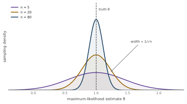
The sketch of why the Normal appears is worth carrying. Near its peak, the log-likelihood looks like a parabola — a second-order Taylor expansion — and a parabolic log-density is exactly a Gaussian. The score \(\ell'(\theta)\) has mean zero at the truth and, being a sum of \(n\) independent terms, is itself approximately Normal by the central limit theorem; dividing by the curvature to solve \(\ell'(\hat\theta)=0\) converts that Normal score into a Normal estimate, and the curvature is what supplies the \(I(\theta)\) in the variance.
A sharper question
If the MLE only reaches the optimal variance as \(n \to \infty\), why trust it at the finite \(n\) I actually have? You often should be cautious — that is the whole next section. The honest claim is asymptotic: efficiency and the clean Normal are large-sample properties, and how large "large" needs to be depends on the model. What buys the reflex is that the approximation improves at a known rate and that maximum likelihood also hands you an estimate of its own uncertainty (the curvature at the peak), so you can at least tell when the sample is too thin to trust the story.
Note
Efficiency is a statement about variance, so it lives inside squared-error thinking, and it is asymptotic and relative to the assumed model. The MLE can be beaten at finite \(n\) by a biased estimator that trades a little bias for less variance — the bias–variance tradeoff of Chapter 12 — and shrinkage estimators (Chapter 13) do exactly this on purpose. "Hard to beat" is a large-sample, correct-model claim, not a universal one.
8.3The failure modes to respect
The guarantees above came wrapped in fine print — "when the model is right," "as \(n\) grows," "well-behaved." Each clause names a way maximum likelihood can mislead you, and a good practitioner knows all three by sight.
Small samples: the MLE is often biased. Consistency says the bias vanishes as \(n \to \infty\), but it says nothing about the sample in front of you. The cleanest example is estimating a Normal's variance. The MLE is \(\hat\sigma^2 = \tfrac1n \sum_i (x_i - \bar x)^2\) — it divides by \(n\). But \(\bar x\) is itself fit from the same data, so the squared deviations are systematically a touch too small, and \(\mathbb{E}[\hat\sigma^2] = \tfrac{n-1}{n}\sigma^2\): the estimate runs low by a factor of \((n-1)/n\). That is why the "sample variance" you were taught divides by \(n-1\), restoring unbiasedness. The MLE is not wrong so much as honest about a different objective — it maximizes likelihood, not unbiasedness — but if you forget the divisor, you will underestimate spread, badly at small \(n\).
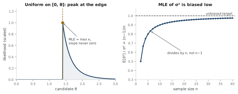
Irregular models: the peak is not where the slope is zero. The whole "set the score to zero, get a Normal" machinery rests on regularity conditions — smoothness of the log-likelihood and, crucially, a data range that does not depend on \(\theta\). The uniform distribution on \([0,\theta]\) breaks the second. Its likelihood is \(\theta^{-n}\) for every \(\theta\) at least as large as the biggest observation and zero below it, so it is increasing-then-cut-off: the maximum sits at the boundary \(\hat\theta = \max_i x_i\), a sharp corner where the derivative never equals zero. The score equation returns nothing useful, and the MLE's distribution is not Normal but a skewed, edge-of-support law — it is even biased, since the sample maximum can only undershoot the true \(\theta\). When a model's support moves with its parameter, discard the smooth story and find the maximum by hand.
Misspecification: the model is wrong. Every guarantee so far assumed the truth lives somewhere in your family of models. When it does not, the MLE does not converge to "the truth" — there is no true \(\theta\) to reach — but to the parameter whose model is closest to reality in Kullback–Leibler divergence, the so-called pseudo-true value. Sometimes that projection is exactly what you want; often it is a confident answer to a question you did not mean to ask. Fit a Normal to data with heavy tails and maximum likelihood will hand you a mean and variance with tight-looking error bars, serenely unaware that the model cannot represent the tails at all.
Common trap
Do not report the maximum-likelihood variance \(\tfrac1n\sum_i (x_i-\bar x)^2\) as "the variance" and move on. It divides by \(n\), so it is biased low, and the smaller your sample the worse the lie. This is not a flaw unique to the variance: fitting a parameter that is itself estimated from the data generically bites into the degrees of freedom, and maximum likelihood does not correct for it on its own.
A sharper question
If the MLE can be biased, irregular, and fooled by the wrong model, why is it the default? Because its failures are legible. The bias is a computable factor you can correct, the irregular cases announce themselves through the model's support, and the misspecification limit has a precise description (the KL projection). An estimator whose breakdowns you can name and bound is more trustworthy than a cleverer one whose failures are opaque — and when the model is right and the sample is large, nothing unbiased beats it. Maximum likelihood is the sensible baseline precisely because you can see the edges of where it works.
Check yourself
A few questions to test the ideas from this chapter. Pick an answer to see whether it holds up.
-
You compute the maximum-likelihood estimate and the likelihood is very high there. What does that high likelihood value actually tell you?
The likelihood is a function of the parameter but a distribution over data, so a high value means the observed data was well anticipated, not that the parameter is probably true. The probability that theta lies somewhere, given the data, is the Bayesian posterior and needs a prior (Chapter 9). A flat prior does make the posterior proportional to the likelihood, but that is a separate, normalized object and the prior may not even be proper. -
The maximum-likelihood estimator of a Normal's variance is the average squared deviation from the sample mean, dividing by n. Compared with the usual sample variance that divides by n minus one, the MLE:
Because the sample mean is fit from the same data, the squared deviations are a touch too small and the expectation is (n-1)/n times the true variance — biased low, worst at small n. Maximum likelihood optimizes likelihood, not unbiasedness, which is why the n minus one divisor is used when unbiasedness is wanted. The bias vanishes as n grows, which is consistency. -
Under regularity conditions, in what precise sense is the MLE hard to beat as the sample grows?
Asymptotic efficiency is a large-sample statement: the MLE becomes approximately Normal around the truth with variance 1/(n I), the lowest an unbiased estimator can reach. It is not a finite-sample claim — a biased estimator can have smaller mean squared error at a given n (Chapters 12 and 13) — and the rate is the ordinary 1/sqrt(n) of the central limit theorem, not faster. -
For the uniform distribution on the interval from 0 to theta, setting the derivative of the log-likelihood to zero fails to locate the MLE. Why, and what is the MLE?
The density is positive only for theta at least as large as every observation, so the likelihood rises to a corner at the sample maximum and is cut off below it — the derivative is never zero there. This violates the regularity condition that the support not move with the parameter, so the MLE is max of the observations, and its distribution is skewed and biased rather than Normal. -
You fit a model by maximum likelihood, but the true data-generating distribution is not a member of your model family. As n grows, the MLE converges to:
With the truth outside the family there is no true theta to reach, so the MLE settles on the pseudo-true value: the model in the family that is nearest the truth in KL divergence. Consistency assumed a correctly specified model, so it does not apply. The danger is that this projection comes with confident-looking error bars for a model that may not represent the data at all.