16Hypothesis Testing

A hypothesis test asks a yes-or-no question of the data: given what you observed, do you keep believing the default story, or do you switch to a rival one? The machinery for answering it, laid down by Jerzy Neyman and Egon Pearson in the 1930s, is not a search for truth but a discipline for acting under uncertainty — a rule that reads the data and returns one of two verdicts, chosen so that its mistakes are controlled at a rate you set in advance. This chapter is about that framing: the two worlds you are deciding between, the two ways a decision can go wrong, and the single statistic — the likelihood ratio — that turns out to be the optimal way to weigh one world against the other.

If you take one idea from this chapter, take this: a test is a decision rule, not a verdict on truth, and the whole theory falls out of one deliberate asymmetry — you cap the rate of the error you fear most, then squeeze the data for as much power against the other as that cap allows.

16.1The Neyman–Pearson framing

Start with two competing accounts of how the data was generated. The null hypothesis \(H_0\) is the default, incumbent story — the coin is fair, the drug does nothing, the two groups have the same mean — the claim you will keep unless the data forces you off it. The alternative hypothesis \(H_1\) is the rival you would switch to. Each hypothesis is a claim about the parameter (Chapter 6) of your model. When a hypothesis pins the distribution down completely — leaving no free parameter, so it names one exact distribution — it is a simple hypothesis; when it only confines the parameter to a set of values, say "the mean is positive," it is a composite hypothesis, a whole family of distributions at once. The cleanest case, and the one the theory solves exactly, is simple against simple.

A test is a rule that partitions the space of possible datasets into two regions: observe data in the rejection region and you reject \(H_0\) in favor of \(H_1\); observe it anywhere else and you fail to reject. That is all a test is — a decision rule (Chapter 11) whose action is one of two labels. And because the data is random, the rule can be wrong in two distinct ways. A Type I error is rejecting \(H_0\) when \(H_0\) is in fact true: a false alarm, convicting an innocent null. Its probability is the size of the test, written \(\alpha\). A Type II error is failing to reject \(H_0\) when \(H_1\) is in fact true: a miss, letting a real effect slip past. Its probability is written \(\beta\). The quantity that gets the attention is not \(\beta\) itself but its complement, the power \(1 - \beta\): the probability that the test does catch a real effect when one is there.

Here is the move that defines the whole framework, and it is a choice, not a theorem. The two errors are not treated symmetrically. You first fix \(\alpha\) at a small value you are willing to tolerate — \(0.05\), \(0.01\) — and only then, among all tests that respect that cap, do you hunt for the one with the largest power. You are not minimizing total mistakes \(\alpha + \beta\); you are minimizing \(\beta\) subject to a hard constraint on \(\alpha\). The decision-theoretic reading (Chapter 11) says why this can be rational: the two errors carry different costs, and \(H_0\) is the hypothesis whose false rejection you have decided is the more expensive blunder — the drug approved that does not work, the effect announced that is not real. Capping \(\alpha\) is a promise about that costly error; maximizing power is doing the best you can about the other, given the promise.

The overlap between the two worlds is what makes the tradeoff unavoidable. If the distribution under \(H_0\) and the distribution under \(H_1\) never overlapped, a single glance at the data would tell you which world you were in and both error rates would be zero. In reality they overlap, and wherever you draw the boundary of the rejection region you are cutting through both densities at once: push the cutoff to shrink the false-alarm area and you enlarge the miss area on the other side. The widget below lets you feel that seesaw directly.

Two words that sound interchangeable are worth pinning apart, because the theory leans on the distinction. The size of a test is its actual worst-case Type I error rate — for a composite null, the largest rejection probability over every parameter value the null allows, \(\sup_{\theta \in H_0} P_\theta(\text{reject})\). The level is the promised upper bound you adopt: a test "has level \(0.05\)" if its size is at most \(0.05\). Size is what the test really does; level is the ceiling you claim for it. They coincide for a well-calibrated test and diverge for a conservative one, whose true size sits below the level it advertises. The best test at a given level is the most powerful test: among all tests of that level, the one whose power against a specified alternative is largest.

16.2The likelihood ratio

Fix a simple null against a simple alternative, and one statistic answers the whole question. The likelihood ratio compares how well each world explains the data you actually saw: \(\Lambda(x) = L_1(x) / L_0(x)\), the likelihood (Chapter 8) of the data under \(H_1\) divided by its likelihood under \(H_0\). A large ratio means the alternative anticipated this data far better than the null did — evidence to switch. The likelihood ratio test rejects \(H_0\) exactly when \(\Lambda(x) \ge k\), with the threshold \(k\) chosen so that the false-alarm rate comes out to \(\alpha\).

The reason this is not merely a reasonable test but the optimal one is the Neyman–Pearson lemma (Neyman & Pearson, 1933): for testing a simple \(H_0\) against a simple \(H_1\), the likelihood ratio test is the most powerful test of its size. No other test that holds the false-alarm rate to \(\alpha\) can achieve higher power. The proof is a greedy argument that is worth carrying as intuition. Think of building a rejection region as spending a fixed budget of Type I error, \(\alpha\), one sliver of the sample space at a time. Each sliver you add to the rejection region costs you its null probability (more \(\alpha\) spent) and buys you its alternative probability (more power). To get the most power per unit of \(\alpha\) spent, you add slivers in order of their bang-for-buck ratio — alternative probability over null probability — which is precisely the likelihood ratio. Threshold the likelihood ratio and you have automatically bought power in the most efficient order possible. That is the lemma.

This is why the likelihood ratio keeps reappearing across statistics — it is the same object you already met as the engine of maximum likelihood (Chapter 8) and, in log form, as the evidence weight behind Bayes factors (Chapter 9). Optimality has a way of making a quantity ubiquitous: once the lemma certifies that ranking the sample space by \(\Lambda\) is the efficient thing to do, every testing problem that can be reduced to that ranking inherits the guarantee.

The lemma is stated for simple against simple, and the natural worry is that real problems are composite: you rarely want to test one exact alternative but rather a whole side of it, like \(H_1: \theta > \theta_0\). Sometimes optimality survives the jump. When the family has a monotone likelihood ratio — the likelihood ratio between any two parameter values is a monotone function of a single statistic \(T(x)\), which every one-parameter exponential family (Chapter 7) enjoys — then the same threshold test on \(T\) is simultaneously most powerful against every alternative on one side at once. Such a test is uniformly most powerful (UMP): most powerful not just against one alternative but uniformly across a composite family of them. This is the Karlin–Rubin theorem, and it is the reason one-sided tests in the standard families have clean, optimal forms. The catch is that UMP tests are fragile: flip to a two-sided alternative \(\theta \ne \theta_0\) and no single threshold can be most powerful in both directions, so a UMP test generally fails to exist.

When exact optimality is out of reach — composite null, composite alternative, several nuisance parameters — you fall back on a general-purpose construction that keeps the likelihood ratio's spirit. The generalized likelihood ratio test replaces each fixed likelihood with the best likelihood its hypothesis can muster: \(\Lambda = \sup_{\theta \in \Theta_0} L(\theta) \,/\, \sup_{\theta \in \Theta} L(\theta)\), the maximized likelihood under the null over the maximized likelihood over the whole parameter space. It compares the best the null can do against the best anyone can do, using maximum likelihood estimates (Chapter 8) to fill in the unknown parameters. Small \(\Lambda\) means the null's best is far worse than the unconstrained best — evidence against \(H_0\).

The obstacle is calibration: how large must \(-2\log\Lambda\) be before you reject? The answer, remarkably, is often free of the specific problem. Wilks' theorem (Wilks, 1938) says that when \(H_0\) is nested inside \(H_1\), then as the sample size grows the statistic \(-2\log\Lambda\) converges in distribution, under the null, to a chi-square distribution whose degrees of freedom equal the number of parameters the null fixes — the difference in dimension between the two models. One null-fixed parameter gives a \(\chi^2_1\) reference curve, two give \(\chi^2_2\), and so on. You compute the statistic, compare it to the appropriate chi-square curve, and read off how extreme it is; the reference distribution came for free, without simulating anything.

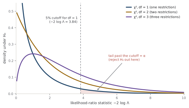
The word asymptotic is load-bearing, and the regularity conditions behind Wilks' theorem are where honest treatments differ from careless ones. The chi-square limit holds only when the models are smoothly parameterized, the null model is genuinely nested in the alternative, the parameters are identifiable, and — the condition most often silently violated — the true parameter lies in the interior of the parameter space under the null, not on its boundary. When the null sits on a boundary, the limit is no longer a clean chi-square. The classic case is testing whether a variance component is zero: because a variance cannot go negative, zero is a boundary, and the correct asymptotic law becomes a mixture of chi-squares — Chernoff's result — often a half-and-half blend of a point mass at zero and a \(\chi^2_1\) (Chernoff, 1954). Treating such a statistic as an ordinary \(\chi^2_1\) makes the test conservative and costs you power. The deeper theory of these limits, and why the chi-square appears at all, belongs to the asymptotics of maximum likelihood (Chapter 19).

References

- Chernoff, H. (1954). On the Distribution of the Likelihood Ratio. The Annals of Mathematical Statistics.
- Neyman, J., & Pearson, E. S. (1933). On the Problem of the Most Efficient Tests of Statistical Hypotheses. Philosophical Transactions of the Royal Society A.
- Wilks, S. S. (1938). The Large-Sample Distribution of the Likelihood Ratio for Testing Composite Hypotheses. The Annals of Mathematical Statistics.
Check yourself
A few questions to test the ideas from this chapter. Pick an answer to see whether it holds up.
-
In the Neyman–Pearson framework you fix the size alpha and then maximize power, rather than minimizing the total error rate alpha + beta. What does this choice actually encode?
Fixing alpha treats the two errors asymmetrically on purpose: rejecting a true null is the error you have decided is worse, so you bound it uniformly over the null and do the best you can on beta. Minimizing alpha + beta is itself well defined and corresponds to a Bayes rule under equal losses and equal priors — its threshold is likelihood ratio = 1 — but that is a different, symmetric problem, which is exactly what Neyman–Pearson declines to assume. -
The Neyman–Pearson lemma guarantees the likelihood ratio test is most powerful. For which testing problem does that guarantee hold exactly?
The lemma is a simple-versus-simple result: both hypotheses must be single, fully specified distributions. It extends to a one-sided composite alternative only under the extra structure of a monotone likelihood ratio (Karlin–Rubin), and that yields a uniformly most powerful test — it is not automatic for every family, and it does not survive two-sided alternatives. -
A test is described as having 'level 0.05' but 'size 0.03'. What is the relationship being expressed?
Size is the supremum of the rejection probability over the null — what the test really does — while level is the ceiling you claim for it; a test has level alpha when its size is at most alpha. A size below the level means the test is conservative and is leaving power on the table. Neither quantity is a Type II rate or a posterior probability of the null. -
You run a generalized likelihood ratio test comparing a full model with 6 free parameters to a nested null that fixes 2 of them. Under Wilks' theorem and its regularity conditions, what is the reference distribution for −2 log Λ?
The degrees of freedom equal the drop in dimension from the full model to the null — the number of restrictions imposed, here 2 — not the total parameter count and not the sample size. Miscounting restrictions mis-calibrates every resulting p-value, and the chi-square itself is only the large-sample limit, valid when the null lies in the interior of the parameter space. -
You test whether a variance component equals zero using −2 log Λ against a chi-square with 1 degree of freedom. A colleague warns the calibration is wrong. Why?
Zero is a boundary for a variance, which violates the interior-point regularity condition behind Wilks' theorem. Chernoff's result gives the correct limit — often a 50:50 mixture of a spike at zero and a chi-square with one degree of freedom — so using the naive chi-square makes the test conservative and costs power. The models here are genuinely nested; the problem is the boundary, not nesting.