2Random Variables and Distributions
Before you can estimate anything, judge a procedure, or trade bias against variance, you need a language for uncertainty — and that language is the distribution. A distribution is not a formula to memorize; it is a bookkeeping device that answers one question in every possible form: where does the probability live? This chapter takes the objects you have already met once — the CDF, the density, the mass function — and shows they are a single thing seen from three angles. Then it asks how distributions combine when you have more than one number to track, and pins down what independence actually buys you.
If you take one idea from this chapter, take this: a distribution assigns a total budget of one unit of probability across the outcomes, and every tool — CDF, density, mass function, marginal, conditional — is just a different way of reading off how that budget is spent.
2.1One object, three views
Start with the thing itself. A random variable is a number whose value is uncertain — formally, a function from outcomes to the real line, but for our purposes just "a measurement you have not made yet." Its distribution is the full account of how likely each value, or range of values, is. That account is the object; the CDF, density, and mass function are three notations for it, each natural in different terrain.
The one notation that always exists is the cumulative distribution function (CDF), written \(F(x) = \mathbb{P}(X \le x)\): the probability that the variable lands at or below \(x\). It sweeps a gate from \(-\infty\) rightward and reports how much probability it has swept past. Because you are accumulating a budget of total size one, \(F\) starts at \(0\), ends at \(1\), and never decreases — those three properties are not just features of the CDF, they are what it means to be a distribution. Every distribution has a CDF, whether the variable is continuous, discrete, or a mix of both. It is the universal view.
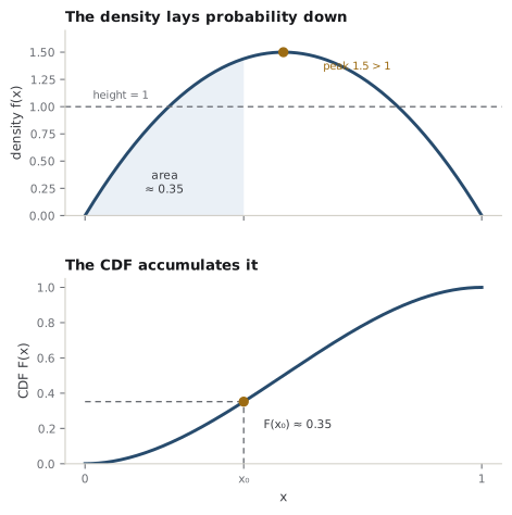
The other two views are derivatives of this one, in both senses. When \(X\) is continuous, its probability density function (pdf) \(f(x)\) is the rate at which the CDF climbs: \(f(x) = F'(x)\), so that probability over an interval is the area underneath, \(\mathbb{P}(a \le X \le b) = \int_a^b f(x)\,dx\). When \(X\) is discrete — it can only land on a countable set of values — its probability mass function (pmf) \(p(x) = \mathbb{P}(X = x)\) places a lump of probability directly on each value, and the CDF becomes a staircase that jumps by \(p(x)\) at each one. Density smears the budget; mass stacks it in piles. Same budget, different bookkeeping.
Intuition
The CDF is the running total; the density (or mass) is the increment. Ask "how much probability by here?" and you want \(F\); ask "how concentrated is it right here?" and you want \(f\) or \(p\). Neither is more fundamental — they are the odometer and the speedometer of the same trip.
Common trap
A density value \(f(x)\) is not a probability. It is a probability per unit of \(x\) — a rate — and rates can exceed one. A distribution tightly concentrated on a narrow interval has a tall density there; the figure's density crests above \(1.5\). What is bounded by one is the area, \(\int f\,dx = 1\), never the height. The moment you read \(f(x)\) as "the chance of \(x\)" you will mispredict, because for a continuous variable the chance of any single exact value is zero.
A sharper question
If the probability of any exact value is zero for a continuous variable, in what sense does the density carry information at all? In the sense of comparisons and intervals. The density says where probability is dense versus sparse: a region where \(f\) is twice as high holds twice as much probability per unit width, so a small interval there is twice as likely. You never consume a density at a point; you integrate it over a set. The point value is a limit — probability of a shrinking window divided by the window's width — and it is that ratio, not any single-point chance, that the density reports.
Why keep three notations for one object? Because each makes a different calculation transparent. The CDF is what you want for "the probability of exceeding a threshold" or for defining quantiles (invert \(F\)). The density is what you integrate to get expectations (Chapter 3) and what you differentiate a likelihood from (Chapter 8). The pmf is the honest description when outcomes are genuinely discrete — counts, categories, successes — where writing a density would be a category error. Fluency is knowing which view collapses your problem to one line.
2.2Joint, marginal, conditional
One variable is rarely the whole story. The moment you track two quantities together — a person's height and weight, a stock's price today and tomorrow — you need the joint distribution, which spends the unit budget of probability over pairs \((x, y)\) rather than single values. In the continuous case it is a joint density \(f(x, y)\), a landscape over the plane whose total volume is one; probability of a region is the volume sitting above it. Everything from one variable generalizes: the joint CDF is \(F(x, y) = \mathbb{P}(X \le x, Y \le y)\), and for discrete pairs a joint pmf puts lumps on grid points.
From the joint you can always recover the behavior of one variable alone by summing out the other. The marginal distribution of \(X\) is what you get by collapsing the joint along the \(Y\) axis — integrating \(y\) away, \(f_X(x) = \int f(x, y)\,dy\) — which is exactly projecting the probability landscape onto the \(x\) axis and reading off its shadow. The name is literal: imagine the joint pmf as a table, and the row and column sums written in the margins are the marginals. Marginalizing answers "forget \(Y\); what does \(X\) do?"
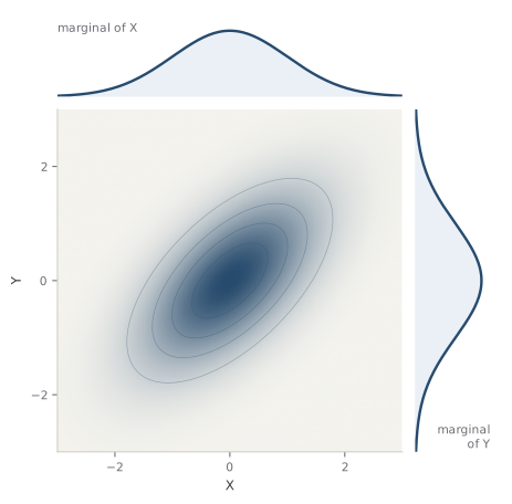
The reverse move is conditioning. The conditional distribution of \(Y\) given that \(X\) took a specific value \(x\) is what remains once you fix \(X = x\) and renormalize: \(f_{Y \mid X}(y \mid x) = f(x, y) / f_X(x)\). Geometrically you slice the joint landscape at \(X = x\), getting a single ridge, then rescale that slice so its area is one again — because within the world where \(X = x\), probability must still sum to a full unit. Conditioning is how new information updates a distribution, and it is the engine of the entire Bayesian view (Chapter 9): a posterior is just a conditional distribution of the unknown given the data.
Analogy
A joint distribution is a topographic map of a mountain range; probability is elevation. The marginal of \(X\) is the range's silhouette seen from the south — every east-west detail flattened into one skyline. The conditional given \(X = x\) is the cross-section you get by slicing the range along one north-south line and looking at that wall face-on. The analogy leaks in the rescaling: a real cross-section keeps its literal height, but a conditional density is renormalized so its own area is one, because it is a fresh distribution over \(Y\), not a raw slice.
These three operations are the complete grammar of combining distributions, and independence is the special case that makes the grammar collapse. Two variables are independent when knowing one tells you nothing about the other — when every conditional equals the corresponding marginal, \(f_{Y \mid X}(y \mid x) = f_Y(y)\) for all \(x\). Substitute that into the definition of conditioning and you get the fact that does all the work:
Independence means the joint factors into its marginals. That is what independence buys you: the shadows determine the whole. In general the marginals badly under-determine the joint — the figure's tilt, the correlation, lives only in the joint and is erased in either shadow — but under independence there is no extra information to lose, and the two one-dimensional descriptions multiply back to the full two-dimensional one.
Intuition
Independence turns a hard high-dimensional object into a product of easy low-dimensional ones. A joint distribution over \(n\) variables is, in general, an \(n\)-dimensional landscape you cannot hope to write down. If the variables are independent, it is just \(n\) separate one-dimensional distributions multiplied together — the curse of dimensionality dodged by assumption.
Note
Independence is strictly stronger than "uncorrelated." Zero correlation only says the joint has no linear tilt; independence says the joint has no structure beyond its marginals at all. You can build variables that are uncorrelated yet fiercely dependent (put probability on a symmetric ring, and \(X\) constrains \(|Y|\) while their correlation is exactly zero). Correlation is one number; independence is a statement about the entire joint density.
A sharper question
Why does the factorization of independence matter so much in practice — isn't it just a tidy formula? Because it is the assumption that makes likelihoods tractable and the limit theorems fire. When you assume your data points are independent and identically distributed (i.i.d.), the joint density of the whole sample is the product of the individual densities, so the log-likelihood is a sum — the form maximum likelihood needs (Chapter 8) and the form the law of large numbers and central limit theorem require (Chapter 5). This same factor-into-a-product move reappears with a twist as the factorization theorem for sufficiency (Chapter 7). Independence is not a tidy formula; it is the hinge the rest of the book swings on.
With distributions in hand as the language, the next chapter asks what you can summarize about one: expectation, variance, and the moments that fingerprint a distribution (Chapter 3). Everything downstream — estimators, risk, the bias-variance tradeoff (Chapter 12) — is built on the account of where probability lives that you have just set up.
Check yourself
A few questions to test the ideas from this chapter. Pick an answer to see whether it holds up.
-
For a continuous random variable, what does the value f(x) of the density at a point x actually represent?
A density is a rate — probability per unit of x — so its height is not capped at one and can be large where probability is concentrated (a Beta(2,2) density crests at 1.5). Probability comes only from area, the integral over an interval. The chance of any single exact value is zero for a continuous variable, and the running total 'at or below x' is the CDF, not the density. -
Which object is guaranteed to exist and fully describe the distribution of any random variable, whether it is continuous, discrete, or a mixture of both?
Only the CDF F(x) = P(X <= x) is universal: it exists for every distribution and characterizes it. A density requires the CDF to be differentiable (continuous case); a mass function requires the variable to be discrete; and a moment generating function need not even exist (some distributions have no finite moments). The CDF is the odometer that always reads out. -
You have the joint density of X and Y. How do you obtain the marginal density of X, and what does it discard?
Marginalizing sums out the other variable — f_X(x) = integral of f(x,y) dy — which projects the joint landscape onto the x axis as its shadow. What vanishes is the dependence structure: correlation and every finer coupling live only in the joint, so two very different joints can share identical marginals. Dividing by f_Y(y) gives a conditional, not a marginal. -
Two random variables are independent exactly when which condition holds?
Independence is the factorization f(x,y) = f_X(x) f_Y(y), equivalently every conditional equals the matching marginal. Zero correlation is strictly weaker — it rules out only linear tilt, and uncorrelated-but-dependent variables are easy to build (put mass on a symmetric ring). Symmetry under swapping is 'exchangeable,' a different property, and knowing the sum generally does constrain each part. -
Why does assuming your data points are independent and identically distributed matter so much for the machinery of later chapters?
Under i.i.d. sampling the joint factors into a product of identical densities, so taking logs turns it into a sum of terms — exactly what maximum likelihood maximizes and what the law of large numbers and central limit theorem average over. The CLT constrains the sum's limit, not the marginals' shape (they need not be normal), and i.i.d. describes sampling with replacement from a fixed distribution, not a census of the population.