11Risk and Decision Theory
You have a procedure — an estimator, a classifier, any rule that turns data into a decision — and you want to know whether it is any good before you run it on a single dataset. You cannot grade it on the answer, because you do not know the truth. What you can do is average its mistake over all the datasets the truth could have produced. That average is the procedure's risk, and the surprise of this chapter is that risk is not one number but a whole curve over the unknown parameter, so "best" turns out to mean three different things depending on how you feel about that curve.
If you take one idea from this chapter, take this: a procedure's risk is a curve over the unknown parameter, and because no single rule sits lowest everywhere, calling one "best" forces you to choose an attitude — beat it everywhere, guard the worst case, or bet on a prior.
11.1Risk as expected loss
Start by naming the thing you are grading. A decision rule \(\delta\) is any function from the observed data \(X\) to an action — for estimation, \(\delta(X)\) is your guess \(\hat\theta\); the estimators of Chapters 6 through 9 are all decision rules, and so is a rule that outputs "reject" or "accept." Chapter 10 gave you a loss function \(L(\theta, a)\) that scores a single action \(a\) against the truth \(\theta\): squared error \((\theta - a)^2\), absolute error \(|\theta - a|\), or 0–1 loss for a decision. The catch is that \(\delta(X)\) is random, because \(X\) is random, so the loss \(L(\theta, \delta(X))\) is a random number you cannot know in advance. The fix is the one move that makes decision theory possible: average the loss over the sampling distribution of the data, the distribution \(X\) follows when the parameter equals \(\theta\).
That average is the risk function:
Read the subscript carefully, because it is the whole point: the expectation is taken with the truth fixed at \(\theta\), over every dataset that value of \(\theta\) could generate. So \(R(\theta, \delta)\) is a function of the unknown parameter — one height for each possible truth. A decision rule does not have a risk; it has a risk curve. Under squared-error loss this curve is exactly the mean squared error of Chapter 12, which is why \(R(\theta, \delta) = \text{bias}(\theta)^2 + \text{variance}(\theta)\) there — the bias-variance split is the risk curve of one particular loss, read pointwise in \(\theta\).
Intuition
Risk is the score a procedure would earn if you replayed the experiment forever at a fixed truth and averaged the mistakes. Since you do not know the truth, you get one such score for every candidate value of it — a curve, not a number — and comparing procedures means comparing whole curves.
Now the comparison. The cleanest thing you can hope for is that one rule's curve sits entirely below another's. Say rule \(\delta_A\) has risk no higher than \(\delta_B\) at every \(\theta\), and strictly lower for at least one \(\theta\); then \(\delta_A\) dominates \(\delta_B\), and there is no reason on earth to use \(\delta_B\) — you can do at least as well everywhere and better somewhere. A rule that some other rule dominates is called inadmissible; a rule that nothing dominates is admissible. Admissibility is the floor, not the ceiling: it only says you cannot be beaten everywhere at once, which is a bar you should insist on but which does not, by itself, pick a winner.
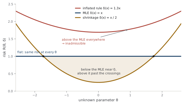
The figure shows the trap in miniature. The inflated rule \(\delta(x) = 1.3x\) is easy to discard: its curve floats above the MLE's flat line everywhere, so it is inadmissible. But the shrinkage rule \(\delta(x) = x/2\) dips below the MLE near \(\theta = 0\) and rises above it in the tails — the curves cross. Neither dominates the other, and this crossing is the normal situation, not a pathology. Most sensible rules are admissible, their curves weaving over and under one another, and admissibility leaves you holding a whole shortlist with no way to rank it.
Common trap
"Admissible" does not mean "good," and "inadmissible" does not always mean "bad." An admissible rule can be terrible everywhere — the constant rule \(\delta(x) = 7\), which ignores the data entirely, is admissible, because no rule beats it at the single point \(\theta = 7\). Admissibility is a purely negative certificate: it rules out being dominated, and nothing more.
A sharper question
If the ordinary estimator has flat, unbeatable-looking risk, surely it is admissible — so why does anyone bother shrinking it? In one dimension the sample mean is indeed admissible, and shrinkage buys only the modest, prior-dependent trade the amber curve shows. The shock, due to Stein, is that in three or more dimensions the ordinary estimator becomes inadmissible: a single shrinkage rule dominates it, cutting risk at every \(\theta\) at once, even for parameters with nothing to do with each other. That is not a tie to be broken by taste; it is strict domination, and it is the whole subject of Chapter 13 (Hastie et al., 2009).
11.2Admissibility, minimax, and Bayes risk
When risk curves cross, admissibility cannot rank them, so you need a way to collapse each curve down to a single comparable number. There are exactly two honest ways to summarize a curve you must commit to before knowing where on it you will land: take its worst value, or take its average value against some weighting. Each yields a criterion, a matching notion of an optimal rule, and — this is the honest part — a different answer, because they encode different attitudes toward the unknown (Wasserman, 2004; Cox, 2006).
The cautious attitude summarizes a curve by its peak. The minimax rule is the one whose worst-case risk is smallest:
You imagine an adversary who, after you pick \(\delta\), sets \(\theta\) to the value that hurts you most — the least favorable value — and you choose the rule that makes that worst case as painless as possible. Minimax buys a guarantee: whatever the truth, your risk is capped at a known level. The price is that you spend all your effort defending against a truth that may be nowhere near reality. A minimax rule often has flat risk, exactly level across \(\theta\), because the way to shrink the maximum of a curve is usually to stop letting it bulge anywhere — spread the risk evenly so no single point can be exploited.
The betting attitude summarizes a curve by its average against a prior distribution \(\pi(\theta)\), the Chapter 9 object encoding how plausible you find each value of \(\theta\) before the data. Averaging the risk curve against the prior gives one number, the Bayes risk:
and the rule that minimizes it is the Bayes decision rule for that prior — also called the Bayes-optimal rule. (This is a different object from "Bayes' rule" the theorem of Chapter 9; the theorem computes a posterior, whereas the Bayes decision rule is the action that minimizes expected loss. Same name, unrelated jobs.) The deep fact is that you do not have to search over all rules to find it. Minimizing the average risk is equivalent to minimizing, for each dataset you might see, the posterior expected loss — so the Bayes decision rule is: observe the data, form the posterior, and output the action that minimizes expected loss under it. Which action that is depends on the loss you chose in Chapter 10: under squared-error loss it is the posterior mean, under absolute-error loss the posterior median, and under 0–1 loss the posterior mode. The loss picks the summary of the posterior; the posterior does the rest.
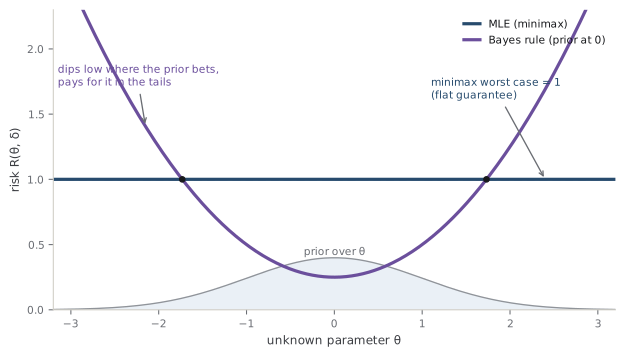
The figure puts the two side by side on the normal-mean problem. The MLE holds its risk flat at one — its worst case is one, and no rule can guarantee lower, so it is minimax. The Bayes rule for a prior centered at zero pulls its risk far down where the prior expects the truth to be, buying a large improvement in the center at the cost of worse-than-minimax risk out in the tails the prior thinks are unlikely. If the truth really is near zero, the Bayes rule wins comfortably; if it is far out, minimax was the safer bet. That is the entire tension of the chapter in one picture.
Common trap
There is no rule that minimizes risk at every \(\theta\) simultaneously — if there were, decision theory would be a footnote. The moment risk curves cross, "the best rule" is undefined until you say by which criterion. Minimax, Bayes, and admissibility are not three routes to one answer; they are three genuinely different answers, and a paper that reports "the optimal estimator" without naming its criterion has quietly smuggled in an attitude toward the unknown.
Analogy
Minimax packs for the worst weather the trip could possibly throw at you; the Bayes rule packs for the forecast. If the forecast is good and holds, the Bayes traveler is lighter and more comfortable the whole way; if a freak storm hits, the minimax traveler is the one who is fine. The analogy leaks where the forecast comes from: a weather forecast is checkable against tomorrow, but a prior is a commitment you make in advance and cannot fully audit — which is exactly why the choice between the two criteria is a choice about temperament, not a fact you can look up.
A sharper question
Isn't minimax just Bayes for a pessimist — and if so, why keep both? The connection is real and beautiful: under broad conditions the minimax rule is the Bayes rule for a particular "least favorable" prior, the prior an adversary would choose to make your life hardest. So minimax is not a rival machinery; it is Bayes aimed at the worst possible prior instead of your honest one. You keep both because they encode different commitments: Bayes says "here is what I actually believe," minimax says "I refuse to assume anything and will insure against the worst." Choosing between them is choosing whether you trust your prior more than you fear the tail.
Note
The three lenses are not fully independent — they lock together at the edges. A Bayes decision rule with respect to a proper prior is, under mild conditions, automatically admissible: if something dominated it, that something would have strictly lower Bayes risk too, contradicting optimality. Admissible rules, in turn, are essentially all Bayes rules or limits of them. So "admissible," "Bayes," and "minimax" are three viewing angles on one geometry, and Stein's inadmissibility result (Chapter 13) is startling precisely because it shows the ordinary estimator falling outside that geometry in high dimensions.
Seen this way, decision theory does not hand you an optimal procedure — it hands you a vocabulary for the fact that optimality is plural. Risk turns a rule into a curve over the unknown; admissibility throws out the curves that are beaten everywhere; and minimax versus Bayes are the two disciplined ways to break the ties that remain, one insuring against the worst case, the other betting on a prior. The next chapter takes the single most important tie-break in the book — the choice to accept a little bias for a lot less variance — and shows that it is not a trick but the shape of the risk curve itself.
References
- Cox, D. R. (2006). Principles of Statistical Inference. Cambridge University Press.
- Hastie, T., Tibshirani, R., & Friedman, J. (2009). The Elements of Statistical Learning: Data Mining, Inference, and Prediction. Springer.
- Wasserman, L. (2004). All of Statistics: A Concise Course in Statistical Inference. Springer.
Check yourself
A few questions to test the ideas from this chapter. Pick an answer to see whether it holds up.
-
The risk of a decision rule is a function of what — that is, what does it assign a number to?
Risk fixes the truth at theta and averages the loss over the sampling distribution, so it returns one height per theta — a curve, not a number. The loss on the sample you drew (the second option) is the random quantity risk averages away; averaging risk against a prior (the fourth) gives the Bayes risk, a single number, which is a later step, not the risk itself. -
A decision rule is inadmissible exactly when:
Inadmissibility means being dominated: beaten weakly everywhere and strictly somewhere. The 'true value' option is a trap — you never know the true theta, so you cannot rank rules by their risk there. Losing on worst-case risk (minimax) or on Bayes risk (Bayes) is a different, weaker kind of loss and does not make a rule inadmissible. -
Minimax rules frequently turn out to have constant risk across the whole parameter space. Why?
Minimizing the peak of a risk curve tends to flatten it — the 'equalizer' intuition — because any point left bulging is a point the adversary aims at. The least-favorable-prior option is the tempting near-miss: a minimax rule often IS Bayes against that prior, but the averaging does not by itself force a flat curve; the equalizing pressure comes from minimizing the maximum. -
You adopt squared-error loss and want the Bayes decision rule. For a given dataset, the action it outputs is:
Minimizing Bayes risk is the same as minimizing posterior expected loss dataset by dataset, and the loss selects the summary: squared error picks the mean, absolute error the median, and 0-1 loss the mode. The MLE option is wrong on two counts — the Bayes rule keeps the prior, and even a flat prior would give the posterior mean, not the mode the MLE tracks. -
Two estimators have risk curves that cross. Which statement is correct?
Crossing curves cannot be ordered by dominance, which is the whole reason minimax and Bayes exist as tie-breakers. Dominance requires one curve weakly below the other everywhere; a smaller worst case is a minimax judgment, not dominance; and intersecting curves can have wildly different Bayes risks depending on where the prior puts mass. -
Under broad conditions, a minimax rule can be re-described in Bayesian terms as:
Minimax is Bayes aimed at the adversary's prior: the least favorable prior is the one maximizing the Bayes risk of its own Bayes rule, and that rule is minimax. A flat prior is a common but wrong guess (least favorable priors are rarely uniform), and the last option describes a rule that dominates all others — which, for crossing curves, cannot exist.