10Loss Functions: What You Are Rewarding
For most of this book the target has been handed to you: estimate the mean, estimate the variance, estimate \(\theta\), and turn the knob until you hit it. But "estimate the parameter" is not yet a question an optimizer can answer, because nothing has said what hitting it is worth or what missing costs. A loss function supplies exactly that — a rule \(L(c, y)\) that scores the penalty for answering \(c\) when the truth is \(y\). Fix a loss and estimation snaps into a well-posed optimization: return the answer with the smallest total penalty. The twist that runs this chapter is that the loss is not a technical afterthought bolted on at the end. It is the steering wheel. Change the loss and the very same data hands you a different "best" estimate.
If you take one idea from this chapter, take this: choosing a loss is a modeling decision about what your mistakes cost, and that choice — not the data — decides which estimate counts as best.
10.1The loss decides the estimate
Ask the simplest estimation question there is. You have a distribution — or just a sample from it — and you must crush it down to a single number \(c\), the best constant summary. Which number? The honest answer is it depends on what a miss costs, and three canonical losses give three genuinely different answers.
Start with squared-error loss, \(L(c, y) = (c - y)^2\), which charges you the square of how far off you are. The best constant is whatever minimizes the expected penalty \(g(c) = \mathbb{E}\big[(c - Y)^2\big]\). Differentiate and set the slope to zero: \(g'(c) = 2\big(c - \mathbb{E}[Y]\big) = 0\), so the minimizer is \(c^\star = \mathbb{E}[Y]\), the mean. Squared error and the mean are the same idea seen twice.
Now switch to absolute-error loss, \(L(c, y) = |c - y|\), which charges you the raw distance, unsquared. Its expected penalty \(\mathbb{E}\big[|c - Y|\big]\) has slope \(\mathbb{P}(Y < c) - \mathbb{P}(Y > c)\): nudging \(c\) upward helps for every point above it and hurts for every point below. That slope is zero exactly when equal mass sits on either side — at the median, the value that splits the distribution into two halves of probability one-half each.
Finally take 0-1 loss, \(L(c, y) = \mathbf{1}[c \ne y]\), which pays nothing for an exact hit and a flat penalty of one for any miss, no matter how large. Since being close counts for nothing, the best you can do is park \(c\) on the single most probable value — the mode, the peak of the density or the most likely category. Three losses, three summaries:
For a symmetric, single-peaked distribution these three coincide, and the choice of loss looks like it does not matter. It is skew and outliers that pull them apart — and then the loss is the whole ballgame. The widget makes the split concrete. It fixes a small sample with one lone outlier and lets you slide the candidate \(c\) while watching two running totals. The squared-loss curve bottoms out at the sample mean; the absolute-loss curve bottoms out at the median. Because the outlier drags the mean well above the median, the two curves reach their lowest points at genuinely different values of \(c\) — the best answer to "summarize this sample" is decided entirely by which loss you picked.
Intuition
The loss is a sentence about what mistakes cost, and the optimal estimate is that sentence read back to you as a number. Squared error says "big misses are catastrophic" and you get the mean; absolute error says "a miss is a miss, count the distance" and you get the median; 0-1 says "only a bullseye counts" and you get the mode.
Analogy
Think of aiming for a bus you must not miss. If arriving early wastes only the minutes you wait but arriving late is a disaster, your loss is lopsided and you leave earlier than the "average" trip would suggest. The loss encodes the consequences of each kind of error, and the best plan bends toward whatever the loss fears most. The analogy leaks in that a bus schedule makes the two costs concrete for you, whereas in estimation you are the one choosing the costs — and different honest choices give different answers.
Common trap
Squared-error loss is not "more accurate" than absolute-error loss, and the mean is not a "better" summary than the median. They optimize different things. Squared error penalizes a large miss out of all proportion to a small one, so its minimizer — the mean — chases any outlier that appears; absolute error weights all misses in proportion to their size, so its minimizer — the median — shrugs the outlier off. Calling one "accurate" smuggles in a loss you never stated. Pick the loss that matches what your mistakes actually cost, and the estimator follows.
10.2The shape of loss and what it forgives
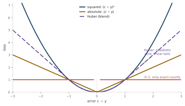
The three summaries above differ because of one thing: the shape of the loss as the error grows. Plot the penalty against the error \(c - y\) and the whole personality of an estimator is visible in the curve. Squared-error loss is a parabola — the penalty grows with the square of the error, so a mistake twice as large hurts four times as much. That steepness is why the mean is so sensitive: a far-flung point contributes an enormous squared penalty, and the only way to relieve it is to slide the estimate toward it. Absolute-error loss is a V — the penalty grows linearly, so a point twice as far away hurts exactly twice as much and no more. A lone outlier gets a vote proportional to its distance, not its distance squared, so it cannot hijack the fit.
That resistance to outliers has a name: robustness, the property that a few extreme or corrupted observations cannot swing an estimate arbitrarily far. Absolute-error loss is robust where squared-error loss is not, and the difference is entirely in how fast the tails of the loss rise (Hastie et al., 2009). But absolute-error loss pays for its robustness with a kink at zero that makes it wobble on small errors and lose a little efficiency when the data really is clean and Gaussian. You would like the graceful small-error behavior of the parabola and the tame tails of the V at once.
Huber loss is exactly that compromise: it is quadratic for residuals smaller than a threshold \(\delta\) and switches to linear beyond it, stitched together so the curve and its slope match at the join (Huber, 1964). Near the center it behaves like squared error, keeping full efficiency on the bulk of well-behaved points; out in the tails it behaves like absolute error, so a gross outlier is charged a linear toll instead of a quadratic one and cannot dominate. The threshold \(\delta\) is a dial: push it to infinity and Huber loss becomes pure squared error, pull it to zero and it becomes pure absolute error. 0-1 loss sits at the far opposite extreme of forgiveness — it is flat, charging the same penalty for a near miss as for a wild one, caring only whether you were exactly right.
A sharper question
If the mean chases outliers, why is squared-error loss the overwhelming default? Three reasons, none of them "it is most accurate." It is smooth, so gradients are easy and the optimization is convex and fast; its minimizer is the mean, which behaves beautifully under averaging and linear operations; and under a Gaussian model it is the maximum-likelihood loss (Chapter 8), so it is optimal precisely when the data has no heavy tails to worry about. Squared error is the right default when your errors are genuinely light-tailed — and a liability the moment they are not. Knowing which world you are in is the actual skill.
Note
Squared-error loss is also the loss under which the tidy MSE = bias² + variance identity holds, which is why the bias-variance tradeoff of Chapter 12 is a fact about squared error specifically. Change the loss and that clean decomposition no longer applies; robustness and the bias-variance split are two different lenses on the same act of choosing a loss.
10.3Aiming off-center with quantile loss
Every loss so far has been symmetric — over-shooting and under-shooting by the same amount cost the same. But plenty of real decisions are lopsided. Overstocking a warehouse wastes storage; understocking loses a sale, and the two rarely cost alike. A loss that treats the two directions differently will aim off-center on purpose, and the tool for it is quantile loss, also called pinball loss. For a chosen level \(\tau\) between \(0\) and \(1\), it charges a residual \(r = y - c\) a slope of \(\tau\) when you under-predict (\(r > 0\)) and a slope of \(1 - \tau\) when you over-predict (\(r < 0\)):
It is a tilted V, and the tilt is the whole point. At \(\tau = 0.5\) the two slopes are equal, the V is symmetric, and you are back to absolute-error loss and the median. Push \(\tau\) up to \(0.9\) and under-prediction is charged nine times as steeply as over-prediction, so the minimizer climbs until only ten percent of the mass lies above it — the \(0.9\) quantile. In general the value that minimizes expected pinball loss at level \(\tau\) is exactly the \(\tau\)-quantile of the distribution (Koenker & Bassett, 1978). Choosing \(\tau\) is choosing which quantile you want to estimate, and it is the same move as before: a statement about what your two kinds of mistake cost, read back as an estimate.
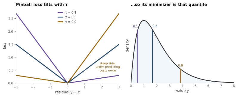
This is how prediction intervals get built without ever assuming a Gaussian: fit the \(0.05\) and \(0.95\) quantiles directly, each with its own pinball loss, and the gap between them is a ninety-percent band. It is a clean example of the chapter's thesis. The estimator you get is not discovered in the data; it is specified by the loss, and swapping the loss swaps the target, cleanly and on purpose.
A sharper question
If the loss just gets averaged over the data anyway, is the choice of loss really separate from the choice of model? Yes, and keeping them separate is what the next chapter is built on. The model says which distributions could have produced the data; the loss says how you will be graded once you commit to an answer. The quantity that fuses them is risk, the expected loss of a procedure averaged over the data it might see — the yardstick for comparing whole procedures before any data arrives, and the subject of Chapter 11. Loss is the per-mistake price; risk is the bill you expect to pay. This chapter fixed the price list; the next one totals the bill and asks which procedure keeps it lowest.
References
- Hastie, T., Tibshirani, R., & Friedman, J. (2009). The Elements of Statistical Learning: Data Mining, Inference, and Prediction. Springer.
- Huber, P. J. (1964). Robust Estimation of a Location Parameter. The Annals of Mathematical Statistics.
- Koenker, R., & Bassett, G. (1978). Regression Quantiles. Econometrica.
Check yourself
A few questions to test the ideas from this chapter. Pick an answer to see whether it holds up.
-
The best constant summary under absolute-error loss is the median rather than the mean. Which fact about expected absolute loss explains this?
Raising c helps for every point below it and hurts for every point above, so the slope is the difference of those two probabilities; it is zero when half the mass lies on each side, which is the definition of the median. The 2(c − E[Y]) slope is the one for squared error, and it lands on the mean. -
A single gross outlier is added to a fixed sample. What happens to the squared-error minimizer and the absolute-error minimizer?
Squared loss charges an outlier the square of its distance, so relieving that penalty drags the mean arbitrarily far; absolute loss charges only the distance, so the outlier gets a bounded vote and the median is essentially unmoved. This bounded influence is exactly what 'robustness' names. -
A colleague says squared-error loss produces a 'more accurate' estimate than absolute-error loss. What is the right correction?
Calling one loss 'accurate' smuggles in an unstated cost structure. The two minimize different functionals — the mean and the median — and which you want depends on what your mistakes cost, not on any intrinsic accuracy ranking. -
Huber loss is quadratic for small residuals and linear for large ones. What does that shape buy?
The quadratic core keeps the good small-error behavior of squared loss where the data is clean, and the linear tails cap an outlier's influence the way absolute loss does. The threshold is a genuine dial: sending it to infinity recovers squared error, to zero recovers absolute error. -
Pinball (quantile) loss with parameter tau = 0.9 does what?
The slopes are tau and 1 − tau, so at tau = 0.9 the ratio is nine to one against under-prediction; the minimizer climbs until only ten percent of the mass lies above it — the 0.9 quantile. Sweeping tau from 0 to 1 traces the whole distribution one quantile at a time. -
Under 0–1 loss, the optimal constant summary of a distribution is its mode. Why the mode rather than the mean or median?
Because a near miss and a wild miss are charged identically, being close earns nothing; the only way to lower expected loss is to raise the chance of an exact hit, which means parking on the peak of the density. This is why classification uses the most-probable-class rule.