20The Bootstrap
Almost everything you want to know about an estimator lives in its sampling distribution: the spread that becomes a standard error, the tails that become a confidence interval, the shape that tells you whether a normal approximation is safe (convergence and the limit theorems, Chapter 5; what makes a good estimator, Chapter 6). For the sample mean you can write that distribution down, because the central limit theorem hands it to you. For the median, a correlation, a ratio of two means, the 90th percentile of a fitted curve, or the cross-validated error of a model, you often cannot — the algebra is a wall. The bootstrap, introduced by Efron in 1979, walks around the wall by a trick that sounds too cheap to work: it manufactures the sampling distribution by resampling the data you already have (Efron, 1979).
If you take one idea from this chapter, take this: the sampling distribution you wish you had comes from the population you cannot see, so the bootstrap substitutes the sample for the population and lets the computer draw the repeated experiments you could not afford — honest wherever the statistic depends smoothly on the distribution, and quietly wrong where it does not.
20.1Resampling to fake a sampling distribution
Start with what you are missing. A statistic \(\hat\theta = s(X_1, \dots, X_n)\) has a sampling distribution — the distribution of the values it would take across the many datasets you never collected — and that distribution is a property of the unknown population \(F\) from which your data were drawn. If you knew \(F\), you could get the sampling distribution to any precision you liked: draw a fresh sample of size \(n\) from \(F\), recompute \(\hat\theta\), repeat ten thousand times, and read off the histogram. The obstacle is the whole problem of statistics. You do not know \(F\); a single sample is all you have.
Efron's move is to plug in the best estimate of \(F\) you own and proceed as if it were the truth. The empirical distribution \(\hat F_n\) is that estimate: it places probability mass \(1/n\) on each of your observed data points and nothing anywhere else, so "drawing from \(\hat F_n\)" just means picking one of your \(n\) points uniformly at random. It is a spiky, discrete caricature of the smooth \(F\) that generated the data, but it is a good caricature — the Glivenko–Cantelli theorem says \(\hat F_n\) converges uniformly to \(F\) as \(n\) grows, so the caricature sharpens into the real thing. This is the plug-in principle: any quantity you would compute from \(F\) if you had it, estimate by computing the same quantity from \(\hat F_n\) instead.
The sampling distribution of \(\hat\theta\) is exactly such a quantity — a functional of \(F\) — so the plug-in principle says to read it off \(\hat F_n\). There is no formula for that functional, but there does not need to be one, because you can simulate it the same way you would have simulated from the true \(F\): draw samples, recompute, repeat. Drawing a sample of size \(n\) from \(\hat F_n\) means drawing \(n\) of your data points uniformly with replacement — a resample, or bootstrap sample. That is the entire nonparametric bootstrap, the version that assumes nothing about the shape of \(F\):
- Draw \(n\) points from your data with replacement; call this resample \(X^*_1, \dots, X^*_n\).
- Recompute the statistic on the resample: \(\hat\theta^* = s(X^*_1, \dots, X^*_n)\).
- Repeat \(B\) times to collect \(\hat\theta^*_1, \dots, \hat\theta^*_B\).
The histogram of those \(B\) values is the bootstrap's estimate of the sampling distribution of \(\hat\theta\), and everything else is bookkeeping on it.
The first thing you read off the histogram is a standard error. The bootstrap standard error is simply the standard deviation of the replicates \(\hat\theta^*_1, \dots, \hat\theta^*_B\) — an estimate of how much \(\hat\theta\) would wobble from dataset to dataset, obtained without a single line of delta-method algebra. For the sample mean it reproduces the textbook \(s/\sqrt{n}\); for a statistic whose standard error you could never derive by hand, it is often the only route to a number at all.
Intuition
The bootstrap treats your sample as a miniature population and asks the question you cannot ask of the real one: if this were the whole world, how much would my estimate jump around as I redrew the data? The wobble of \(\hat\theta^*\) around \(\hat\theta\) in the resamples stands in for the wobble of \(\hat\theta\) around the true \(\theta\) across real samples. The substitution is honest to the exact degree that your sample resembles the population — which is why it improves with \(n\) and cannot be trusted when \(n\) is tiny.
Two different approximations are stacked here, and keeping them apart is the key to using the bootstrap well. The first is statistical: you replaced \(F\) with \(\hat F_n\), and how good that is depends on the sample and is out of your hands once the data are collected. The second is Monte Carlo: you used \(B\) resamples instead of the infinitely many the plug-in principle really refers to, and this one is entirely under your control — push \(B\) into the thousands and the Monte Carlo error all but vanishes, leaving only the statistical error that actually limits you. Confusing the two leads people to think a huge \(B\) rescues a bad bootstrap; it does not, because \(B\) never touches the gap between \(\hat F_n\) and \(F\).
A sharper question
Why does resampling with replacement, not without, matter — isn't sampling without replacement more like collecting fresh data? Without replacement is a trap that gives you nothing. Drawing \(n\) points from \(n\) without replacement returns your original sample in a shuffled order every single time, so every \(\hat\theta^*\) equals \(\hat\theta\) and the bootstrap distribution collapses to a spike with zero spread. Sampling with replacement is what makes each resample a genuinely new draw of size \(n\) from \(\hat F_n\) — some points appear twice or thrice, others are left out (about \(e^{-1} \approx 37\%\) of them, on average) — and that reshuffling of multiplicities is precisely what mimics the variation of drawing a fresh sample from the population. The variability you want is manufactured by the repetition, so removing the repetition removes the point.
From the same \(B\) replicates you can build a confidence interval, and there are three flavors worth knowing, in increasing order of care (confidence and credible intervals, Chapter 18). The percentile interval is the bluntest: take the empirical \(2.5\)th and \(97.5\)th percentiles of the bootstrap replicates and call that your \(95\%\) interval. The basic, or pivotal, interval instead treats \(\hat\theta^* - \hat\theta\) as a stand-in for the sampling error \(\hat\theta - \theta\) and reflects the percentiles back through the estimate, giving endpoints of the form \(2\hat\theta - q_{97.5}\) and \(2\hat\theta - q_{2.5}\); this fixes the percentile interval's habit of pointing the wrong way when the bootstrap distribution is shifted off-center. The BCa interval — bias-corrected and accelerated, from Efron 1987 — is the refined default: it adjusts the percentile endpoints by two data-driven numbers, a bias correction \(z_0\) that recenters when \(\hat\theta\) sits off the median of its own bootstrap distribution, and an acceleration \(a\) that accounts for a standard error that changes with \(\theta\) (skewness) (Efron, 1987). Those two corrections buy second-order accuracy: the interval's true coverage approaches the nominal \(95\%\) at rate \(1/n\) rather than the \(1/\sqrt{n}\) of the plain percentile interval, an improvement that Edgeworth-expansion arguments make precise and that matches the accuracy of a hand-tuned analytic interval without the hand-tuning (Singh, 1981).
Note
Why does simple resampling deliver an accuracy that a normal approximation misses? Because the bootstrap distribution automatically carries the skewness of the statistic's true sampling distribution, which the symmetric normal approximation throws away. An Edgeworth expansion writes the sampling distribution as a normal plus correction terms in powers of \(1/\sqrt{n}\); the first correction is a skewness term, and the bootstrap reproduces it from the data rather than assuming it is zero. That single recovered term is the whole source of the bootstrap's edge over textbook normal intervals — and it is why BCa, which corrects skewness explicitly, beats the percentile interval, which does not.
The reason any of this is legitimate rather than a sleight of hand is a genuine theorem, not a hope. For a broad class of statistics — smooth functions of sample means, and more generally functionals that vary smoothly with the distribution — the bootstrap distribution converges to the true sampling distribution as \(n\) grows, so the interval you read off it has the coverage it claims in the limit (Bickel & Freedman, 1981). This is the sense in which "using the data as its own population" is honest: not because \(\hat F_n\) equals \(F\), but because the quantity you actually care about, the shape of the sampling distribution, is recovered in the limit even though \(F\) itself is only approximated. The consistency is asymptotic and it is conditional on smoothness — two caveats the next section turns into the failure cases you must respect.
A sharper question
Is the bootstrap giving me a frequentist or a Bayesian interval? Frequentist, squarely. It approximates the repeated-sampling behavior of \(\hat\theta\) — how the estimate would vary across hypothetical new datasets — which is exactly the frequentist notion of a sampling distribution, and its intervals are justified by coverage under repeated sampling, not by a posterior (the Bayesian view, Chapter 9). The resemblance to a posterior is real but a coincidence of asymptotics: there is a Bayesian bootstrap that reweights the data with random Dirichlet weights and does yield a posterior under a particular noninformative prior, and in large samples the ordinary percentile interval and a flat-prior credible interval often nearly coincide — the same convergence that makes maximum likelihood and Bayes agree asymptotically. But the ordinary bootstrap answers a frequentist question, and reading its interval as "a \(95\%\) probability that \(\theta\) is in here" imports a Bayesian meaning the method never promised.
20.2What it can and cannot do
The consistency theorem came with a word in it — smooth — and the bootstrap's failures are all that word failing. When the statistic depends on the population through an average, a smooth function of averages, or any functional that a small change in the distribution nudges gently, the bootstrap works and works well. When the statistic hinges on a feature that a small change in the distribution can move discontinuously — an extreme, a boundary, an infinite moment — the plug-in substitution breaks, and it breaks in ways that more data does not repair. The honest skill is knowing which case you are in before you trust the interval.
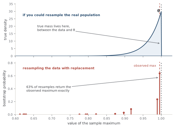
The cleanest failure is the sample maximum. Suppose your data are drawn from a uniform distribution on \([0, \theta]\) and you estimate the ceiling \(\theta\) by the largest observation \(\hat\theta = X_{(n)}\). The true sampling distribution of \(X_{(n)}\) is smooth: across real samples the maximum lands at various values just below \(\theta\), spread out in a tidy density (the sampling distribution, Chapter 5). The bootstrap distribution is nothing like it. Every resample is drawn from your data, so no resample can ever contain a value larger than the observed maximum — the bootstrapped maximum is pinned at or below \(X_{(n)}\), and in fact it equals \(X_{(n)}\) in about \(63\%\) of resamples (any resample that happens to include the top point, which is \(1 - (1 - 1/n)^n \to 1 - e^{-1}\)). The result is a lumpy distribution with a huge atom on the observed maximum and smaller atoms on the next few order statistics, and it does not converge to the smooth truth no matter how large \(n\) becomes. The bootstrap is not merely inaccurate here; it is inconsistent.
A sharper question
Why does the bootstrap fail for the sample maximum when it works for the sample mean? Because the maximum is a non-smooth functional pinned to the edge of the data, and resampling can only recycle values that are already inside the sample. The mean is an average, so a resample can push it slightly above or below \(\hat\theta\) in either direction, faithfully mimicking how the real mean varies; the maximum can only stay at the observed top value or drop to a lower one, so the resampled distribution is one-sided and clotted onto points, structurally unable to reproduce a smooth density that lives partly above the observed maximum. The deep reason is that the true limiting law of an extreme (an extreme-value distribution) depends on the tail of \(F\) beyond your data, exactly the region \(\hat F_n\) knows nothing about — the empirical distribution has a hard wall at \(X_{(n)}\) and puts zero probability past it. This is the boundary case in general: whenever the parameter sits on the edge of its space or the statistic is governed by the unobserved tail, the plug-in substitution loses the very information the answer depends on.
The same crack runs under two other situations that look different but share the diagnosis. The first is heavy tails: when \(F\) has infinite variance, the sample mean has no central-limit normal to converge to, and the bootstrap of the mean inherits the pathology — its distribution is driven by a few extreme points that appear a random number of times across resamples, and it fails to consistently estimate the (non-normal) sampling distribution. The second is dependent data: a time series or a spatially correlated sample carries structure between neighboring observations, and resampling points independently — which is what drawing from \(\hat F_n\) does — shatters that structure, throwing away the autocorrelation and badly underestimating the true variance.
Common trap
The ordinary bootstrap silently assumes your observations are independent and identically distributed, and applying it to correlated data is one of the most common ways to get a confidently wrong standard error. Because independent resampling destroys the serial dependence, the bootstrap treats a smooth, autocorrelated series as if it carried far more independent information than it does, and it reports a standard error that can be several times too small — an interval that looks reassuringly tight and is simply false. The fix is the block bootstrap (Künsch 1989), which resamples contiguous blocks of consecutive observations rather than single points, so the dependence inside each block is preserved and only the weaker dependence across blocks is broken (Künsch, 1989). Choosing the block length is its own small art — too short and you lose the dependence you were trying to keep, too long and you have too few blocks to resample — but the principle is simply to resample the unit that carries the correlation.
There is a family of repairs for the boundary and heavy-tail failures too. The m-out-of-n bootstrap resamples \(m\) points rather than \(n\), with \(m\) growing slower than \(n\), and subsampling schemes like it restore consistency in several cases where the ordinary bootstrap is inconsistent — including the sample maximum — by drawing resamples small enough that the plug-in error washes out (Bickel et al., 1997). These are specialist tools, but they are worth knowing exist: the failure of the plain bootstrap is not the end of resampling, only a signal that the naive version is the wrong one.
When you are willing to assume a model, the parametric bootstrap is often the better instrument. Instead of resampling from the empirical distribution, you fit a parametric family — estimate \(\hat\theta\), say by maximum likelihood (Chapter 8) — and then simulate fresh datasets from the fitted distribution \(F_{\hat\theta}\), recomputing the statistic on each. Where the nonparametric bootstrap resamples the data, the parametric bootstrap resamples from a smooth fitted curve, which sidesteps the spiky \(\hat F_n\) entirely and can be far more efficient when the model is right — and it can even rescue the boundary case, because a fitted uniform on \([0, \hat\theta]\) can generate values above the observed maximum. The catch is exactly the model: the parametric bootstrap is only as trustworthy as the family you assumed, and it inherits every bias of a misspecified model, whereas the nonparametric version buys its robustness by assuming almost nothing.
Common trap
A small sample makes the bootstrap unreliable in a way no amount of computing fixes, and this is easy to forget because the method runs happily on any \(n\). With \(n = 10\), the empirical distribution is a crude, ten-spike approximation to \(F\), so the bootstrap standard error inherits that crudeness — and a bootstrap distribution built from a handful of points can only take a handful of distinct values, giving intervals with visibly granular, undependable coverage. Cranking \(B\) up to a million does nothing, because the limit is the statistical gap between \(\hat F_n\) and \(F\), not the Monte Carlo count; the honest response to small \(n\) is a modeling assumption (a parametric bootstrap) or humility, not a bigger resampling loop.
So the bottom line is a rule with a reason, not a superstition. Trust the bootstrap for smooth functionals of the distribution — means, variances, correlations, regression coefficients, quantiles away from the extreme edges, model error estimates — at moderate-to-large \(n\) with finite variance and roughly independent data, where the consistency theorem applies and the second-order accuracy of BCa is real (asymptotic efficiency, Chapter 19). Distrust it, or reach for a specialized variant, at the extremes and boundaries, under heavy tails, under serial or spatial dependence, and at small \(n\) — the places where a small change in the distribution moves the answer discontinuously, or where the sample is too thin to stand in for the population. The bootstrap's reputation as a free lunch is deserved across a genuinely wide range of problems, and knowing where the lunch stops being free is the difference between a tool and a talisman — a distinction that only sharpens as the models grow and the parameters outnumber the data (high-dimensional phenomena, Chapter 21).
References
- Bickel, P. J., & Freedman, D. A. (1981). Some Asymptotic Theory for the Bootstrap. The Annals of Statistics.
- Bickel, P. J., Götze, F., & van Zwet, W. R. (1997). Resampling Fewer Than n Observations: Gains, Losses, and Remedies for Losses. Statistica Sinica.
- Efron, B. (1979). Bootstrap Methods: Another Look at the Jackknife. The Annals of Statistics.
- Efron, B. (1987). Better Bootstrap Confidence Intervals. Journal of the American Statistical Association.
- Künsch, H. R. (1989). The Jackknife and the Bootstrap for General Stationary Observations. The Annals of Statistics.
- Singh, K. (1981). On the Asymptotic Accuracy of Efron's Bootstrap. The Annals of Statistics.
Check yourself
A few questions to test the ideas from this chapter. Pick an answer to see whether it holds up.
-
The nonparametric bootstrap is inconsistent for the sample maximum of data on the interval from 0 to theta. What is the essential reason?
The maximum is a non-smooth functional pinned to the data's edge: the empirical distribution has a hard wall at the observed maximum and zero mass beyond it, so resamples clump onto the order statistics (about 63% return the observed maximum exactly) and cannot converge to the true extreme-value law, which depends on the unobserved tail. The bootstrap routinely handles biased statistics and even estimates bias, so B is a red herring; here the variance is finite. The m-out-of-n bootstrap restores consistency. -
Why must bootstrap resampling draw n points WITH replacement rather than without?
Drawing n points with replacement is exactly drawing an i.i.d. sample of size n from the empirical distribution: some points repeat, about 37% are omitted, and that reshuffling of multiplicities manufactures the variability that mimics collecting a fresh sample. Without replacement, a full draw just reorders the data, so there is no variation at all. Resamples are not required to be distinct, and the empirical distribution can be sampled either way in principle; it is the full without-replacement draw that is degenerate. -
You run a bootstrap with B = 200 resamples and get a jagged interval. A colleague says 'just use B = 100,000.' When does that help?
Two approximations are stacked: the Monte Carlo error from using finitely many resamples, which a large B drives to nearly zero, and the statistical error from replacing the true distribution with the empirical one, which is fixed once the data are collected. Raising B never touches the second gap, so it cannot compensate for small n or add information about theta. It only removes the simulation noise, leaving the statistical error that actually limits the interval. -
The BCa interval is 'second-order accurate' while the plain percentile interval is only first-order accurate. What does the extra order buy, and why?
An Edgeworth expansion writes the sampling distribution as a normal plus corrections in powers of 1/sqrt(n); the first correction is a skewness term. BCa's bias correction and acceleration recover that term from the data, so its coverage error falls like 1/n rather than 1/sqrt(n). It is not about interval length, it is still an asymptotic (not exact) guarantee, and it does nothing to rescue non-smooth statistics like the maximum. -
Applied to a strongly autocorrelated time series, the ordinary i.i.d. bootstrap tends to report standard errors that are:
Resampling points independently shatters the autocorrelation, so the bootstrap acts as if the series carried far more independent information than it does and reports a standard error that can be several times too small. The block bootstrap fixes this by resampling contiguous blocks of consecutive observations, preserving the dependence inside each block. The i.i.d. bootstrap is not distribution-free with respect to dependence: independence is a built-in assumption. -
When would you prefer the parametric bootstrap (simulating from a fitted model) over the nonparametric one (resampling the data)?
The parametric bootstrap replaces the spiky empirical distribution with a smooth fitted one, so it is more efficient when the model is right and can even escape the boundary failure (a fitted uniform can produce values above the observed maximum). Its price is model dependence: it inherits every bias of a misspecified family. It is not simply cheaper, large n makes the empirical distribution better rather than worse, and the ordinary bootstrap is frequentist, not Bayesian (the Bayesian bootstrap is a separate, Dirichlet-weighted method).