12The Bias–Variance Tradeoff
Every estimate you will ever make is wrong. The only interesting question is how it is wrong — and it turns out there are exactly two ways, which pull against each other. This chapter is about that split, because once you see it, regularization, shrinkage, and a good chunk of modern statistics stop looking like tricks and start looking inevitable.
If you take one idea from this chapter, take this: an estimator's error breaks into bias and variance, and buying down one usually costs you the other.
12.1Decomposing the error
Fix a quantity you want to estimate — call it \(\theta\) — and an estimator \(\hat\theta\) built from your data. Because the data is random, \(\hat\theta\) is random too: draw a fresh sample and you get a fresh value. Measure how wrong it is by the mean squared error, the expected squared distance from the truth:
Add and subtract the estimator's own average value \(\mathbb{E}[\hat\theta]\), expand the square, and the cross term drops out (its expectation is zero). What remains is exact, and worth committing to memory:
Intuition
Bias is how far off you are on average; variance is how much you jitter around that average. Total error adds the two — miss the center or spray your shots, and either way you pay.
Analogy
Throwing darts. Bias is the gap between the center of your cluster and the bullseye; variance is how spread out the cluster is. A tight cluster in the wrong place (low variance, high bias) and a loose cluster around the center (low bias, high variance) can be equally bad. The analogy leaks in one place, noted just below.
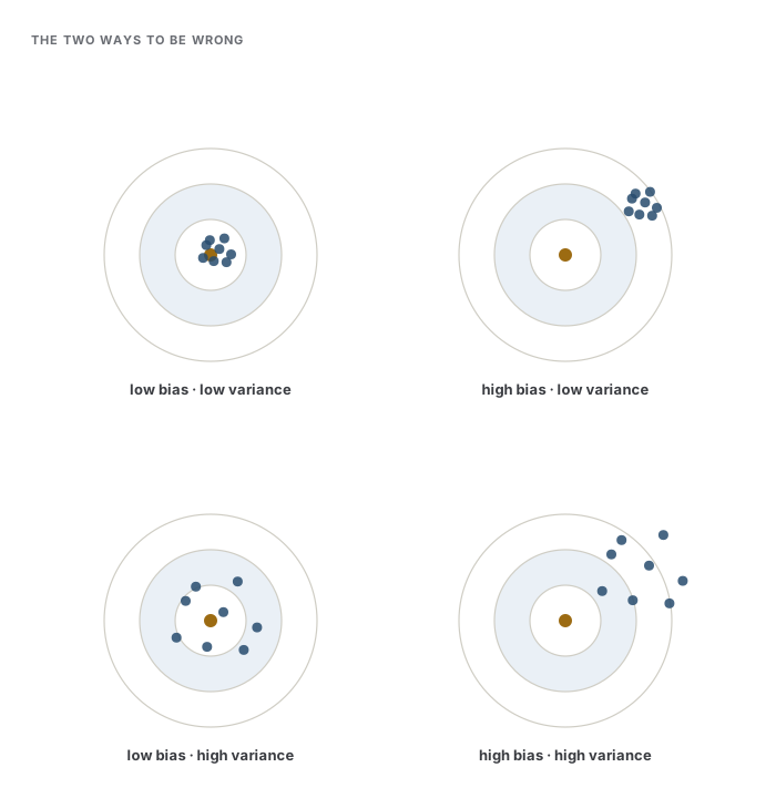
The dartboard makes the two failure modes vivid, but it hides the thing that makes statistics interesting. Where does the analogy leak? A skilled dart thrower could, in principle, be both accurate and precise — top-left, no compromise. An estimator usually cannot: the very knob that steadies your aim also tugs it off-center. That forced trade is the rest of the chapter.
12.2Why a little bias can help
Because MSE is bias squared plus variance, minimizing error is not the same as minimizing bias. An unbiased estimator zeroes the first term, but nothing stops the second from being enormous. If you can swallow a pinch of bias and cut variance by more, total error goes down.
That is exactly what regularization does, and the cleanest possible example shows it in closed form. You observe a single number \(z\) whose mean is the unknown \(\beta\) and whose variance is \(\sigma^2 = 1\). The obvious estimate is \(z\) itself — unbiased, done. But consider shrinking it toward zero by a penalty \(\lambda\):
This is ridge regression stripped down to one dimension. Its bias climbs with \(\lambda\) and its variance falls with \(\lambda\), and their sum is a U:
Slide the penalty below and watch the three curves move. At \(\lambda = 0\) you are unbiased and pay full variance. Push \(\lambda\) up and bias takes over. Somewhere in between, the total dips below its unbiased value — the shrunk estimate beats the obvious one.
The minimum sits at \(\lambda^{*} = \sigma^{2}/\beta^{2}\): shrink harder when the noise is loud relative to the signal, and less when the signal is strong.
A sharper question
If shrinking toward zero is biased, why does it ever beat the unbiased estimate — isn't zero an arbitrary place to pull toward? For a single number it is fairly arbitrary, and the win is modest. What makes shrinkage a deep idea rather than a lucky accident is that when you estimate many parameters at once, pulling them toward a common center beats estimating each on its own — even when the parameters have nothing to do with each other. That is Stein's paradox, and it is the whole of the next chapter (Hastie et al., 2009).
Common trap
The tidy identity MSE = bias² + variance is a fact about squared-error loss. Switch the loss — to absolute error, say — and the clean split no longer holds. When someone invokes "the bias-variance tradeoff," they are almost always standing inside squared-error loss, whether or not they say so.
The tradeoff is the lens for all of Part IV. Every regularization method — ridge, lasso, early stopping, a Bayesian prior — is a way of choosing where on the bias-variance curve to stand. What is left is deciding how far to shrink, which is where cross-validation and the effective degrees of freedom come in.
References
- Hastie, T., Tibshirani, R., & Friedman, J. (2009). The Elements of Statistical Learning: Data Mining, Inference, and Prediction. Springer.
Check yourself
A few questions to test the ideas from this chapter. Pick an answer to see whether it holds up.
-
Under squared-error loss, the mean squared error of an estimator of a fixed parameter decomposes into exactly two pieces. What are they?
For squared-error loss, MSE = (bias)^2 + variance — a clean, exact identity, not an approximation, because the cross term in the expansion has expectation zero. Bias and standard deviation are in different units and cannot be added, and the irreducible noise term appears only when you predict a fresh noisy observation, not when you estimate a fixed parameter. -
A colleague insists on using only unbiased estimators. Why is that not automatically the right call?
MSE trades bias against variance, and the minimum of their sum often sits at a nonzero bias. Pulling an estimate toward a center adds bias but can shrink variance by more, lowering total error — the whole reason regularization works. Unbiased estimators usually do exist; the point is that optimality is about total risk, not about zeroing the bias term. -
As you increase a regularization penalty (shrinking an estimate harder toward zero), what typically happens to bias and variance?
Heavier shrinkage pulls the estimate away from what the data alone would say, raising bias, while making the estimate less sensitive to the particular sample, lowering variance. Total risk is U-shaped in the penalty: too little regularization is all variance, too much is all bias, and the sweet spot lies in between. -
You observe z with mean beta and variance one, and estimate beta by z / (1 + lambda). The risk-minimizing penalty lambda* depends on what?
Minimizing risk gives lambda* = sigma^2 / beta^2: shrink harder when noise is large relative to signal, and less when the signal is strong. It is emphatically not always zero — that is the surprise, since lambda = 0 is the unbiased estimate z, yet a positive penalty lowers risk. And lambda* is a property of the problem, not something read off one observed z. -
'Variance' in the bias-variance decomposition refers to variability of what?
The variance term measures how much the estimator would bounce around if you redrew the data many times — a thought experiment over samples, not a spread visible inside one dataset. Confusing it with the within-sample spread of the data, or with one fit's residuals, is the usual slip; in the frequentist decomposition the parameter is fixed, not random.