21High-Dimensional Phenomena
Every asymptotic result in this book so far has told the same story: fix the number of unknowns, let the sample size \(n\) run to infinity, and watch a good estimator settle onto the truth. That is the world of asymptotic efficiency (Chapter 19), where the maximum-likelihood estimate becomes normal, unbiased, and optimal as data piles up around a handful of parameters. Modern data does not look like that. A genomics study measures twenty thousand genes on a few hundred patients; a text model carries more parameters than it has training tokens. The number of things you are estimating, \(p\), is not a fixed backdrop — it grows right alongside \(n\), often in step with it. High-dimensional statistics is what you get when you take that seriously: you study the regime where \(p\) and \(n\) grow together, typically with their ratio \(p/n\) tending to a constant rather than to zero.
If you take one idea from this closing chapter, take this: when the number of parameters is comparable to the sample size, the estimators you learned to trust do not merely get noisier — they fail in structured, predictable ways, and the shrinkage and regularization the earlier chapters treated as clever options become the only way to estimate at all. The high-dimensional regime is where every thread of the book — distributions, risk, the bias–variance tradeoff, shrinkage — is pulled taut at once.
21.1When p grows with n
Classical asymptotics holds \(p\) fixed and sends \(n \to \infty\), so each parameter eventually drowns in data. The high-dimensional regime instead lets \(p\) scale with \(n\), holding the ratio \(p/n \to \gamma\) for some constant \(\gamma > 0\). The distinction is not pedantic. With \(p\) fixed you have, in effect, \(n/p \to \infty\) observations per unknown; with \(p/n \to \gamma\) you have a bounded number of observations per unknown forever, no matter how large the dataset grows. The law of large numbers and the central limit theorem (Chapter 5) still hold coordinate by coordinate, but the aggregate object you actually care about — a whole covariance matrix, a whole coefficient vector — never gets the averaging-out that fixed-\(p\) theory quietly assumed.
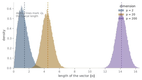
The first thing to break is geometric intuition, and it breaks through concentration of measure: in high dimensions, a function that does not depend too sharply on any single coordinate is almost constant across the randomness, so quantities that feel like they should vary end up pinned to a single typical value. The cleanest case is length. Draw \(X \sim \mathcal{N}(0, I_p)\), a standard Gaussian in \(p\) dimensions. Its squared length \(\lVert X \rVert^2 = \sum_i X_i^2\) has mean \(p\) and standard deviation \(\sqrt{2p}\), so the length \(\lVert X \rVert\) sits almost exactly at \(\sqrt{p}\) with a spread that shrinks relative to \(\sqrt{p}\) as \(p\) grows. The bell curve you picture with a dense center is a lie in high dimensions: essentially all the probability lives in a thin shell of radius \(\sqrt{p}\), and the center — the single most likely point of the density — is empty.
Intuition
In one or two dimensions, "random Gaussian point" means "probably near the origin." In a thousand dimensions it means "almost certainly on the sphere of radius \(\sqrt{p}\), in a direction you cannot predict." Distance stops being informative because everything is about \(\sqrt{2p}\) apart from everything else, and volume crowds so hard toward the surface that the interior effectively vanishes.
This is the same geometry that made shrinkage win in the shrinkage surprise (Chapter 13). There, the noise vector \(X - \theta\) had squared length about \(p\sigma^2\) and landed nearly perpendicular to the truth, so the observed vector overshot \(\theta\) by a predictable amount and pulling it back helped. Concentration is why that story was not a fluke of one example: near-orthogonality of independent directions and the length overshoot are both concentration phenomena, and they only sharpen as \(p\) climbs. Stein's inadmissibility result was the first tremor of high-dimensional statistics, felt in 1956 before anyone used the name (Stein, 1956).
Analogy
Think of an orange. In two dimensions almost all of a disk's area is well inside the rind; in three, more of the volume has crept toward the peel; by a thousand dimensions the fruit is all peel and no flesh, a paper-thin skin holding an empty interior. The analogy leaks in the usual way a picture of high dimensions must: there is no honest way to draw the thousand-dimensional orange, so you are trusting the arithmetic of volumes, not your eyes — which is exactly the discipline high dimensions demand.
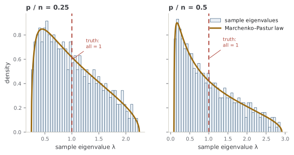
Now watch a workhorse estimator degrade. The sample covariance matrix \(\hat\Sigma = \frac{1}{n} \sum_i X_i X_i^\top\) is the natural estimate of the true covariance \(\Sigma\); in fixed-\(p\) asymptotics it converges to \(\Sigma\) entry by entry and its eigenvalues converge to the truth's. Suppose the truth is the simplest possible, \(\Sigma = I_p\), so every true eigenvalue is exactly \(1\). When \(p/n\) is bounded away from zero, the eigenvalues of \(\hat\Sigma\) do not cluster at \(1\) — they smear out into a whole spread. The limiting shape of that spread is the Marchenko–Pastur law: as \(p, n \to \infty\) with \(p/n \to \gamma\), the histogram of sample eigenvalues converges to a fixed density supported on the interval \([(1-\sqrt{\gamma})^2,\ (1+\sqrt{\gamma})^2]\), even though every eigenvalue of the truth equals \(1\) (Marchenko & Pastur, 1967).
A sharper question
Why does the sample covariance fail when \(p \approx n\), when each individual entry is still an unbiased average that the law of large numbers should tame? Every single entry of \(\hat\Sigma\) is fine — it is an average of \(n\) terms and converges. The failure is collective. You are estimating about \(p^2/2\) covariance parameters from \(n\) vectors, and when \(p^2 \gg np\) there simply is not enough data to pin the matrix down as a whole. The eigenvalues are the tell: they are the most extreme summaries of the matrix, and small correlated errors in many entries conspire to push the top eigenvalue up and the bottom one down. Marchenko and Pastur compute exactly how far. Johnstone later showed the largest eigenvalue's fluctuations follow the Tracy–Widom law, so even the edge of the spread has a precise, non-Gaussian shape (Johnstone, 2001).
The same rot reaches the maximum-likelihood estimate (Chapter 8). Its guarantees of consistency and efficiency were asymptotic in the fixed-\(p\) sense; they assumed each parameter would eventually be swamped with data. When \(p\) grows with \(n\) that never happens, and the MLE can be badly biased, wildly variable, or — for a covariance or a regression with \(p > n\) — not even uniquely defined, because the likelihood is flat along whole directions the data never constrains. The clean picture from Chapter 19, where the MLE rides the Cramér–Rao floor down to zero, is a fixed-\(p\) luxury.
So what do you do when the raw estimator is inadmissible or undefined and every point is far from every other? You stop asking for the unconstrained fit and impose structure — which is exactly what regularization does. Ridge regression and the lasso (Chapters 14 and 15) do not just improve on the high-dimensional least-squares fit; they rescue it, because the least-squares fit with \(p > n\) has infinitely many zero-training-error solutions and no way to choose among them. The most productive structure to assume is sparsity: that although you measured \(p\) features, only a small number \(s \ll p\) of them actually matter, and the rest have true coefficient zero. Under sparsity the lasso comes with a striking guarantee. If the design matrix satisfies a restricted eigenvalue condition — roughly, that it does not collapse the few directions the sparse signal lives in, so those coordinates are not hopelessly tangled with the rest — then the lasso's estimation error is of order \(\sqrt{s \log p / n}\) rather than \(\sqrt{p/n}\) (Bickel et al., 2009). You pay only for the \(s\) coefficients that matter, times a mild \(\log p\) toll for not knowing in advance which \(s\) they were.
A sharper question
What makes sparsity recoverable at all — why should \(s \log p / n\) be achievable when there are \(\binom{p}{s}\) possible support sets to search? Two ingredients. First, the rate says you pay \(\log p\), not \(p\): that logarithm is the price of searching over all \(\binom{p}{s}\) subsets, and it is small because \(\log \binom{p}{s} \approx s \log p\). Second, the restricted eigenvalue condition is doing quiet, essential work. It guarantees that the true sparse signal is not confusable with some dense combination of the other predictors — that the geometry of the design keeps the relevant few directions well separated. Without it, two different sparse models can fit the data equally well and no method can tell them apart; the rate is not a property of the lasso alone but of the lasso on a design that permits recovery. Sparsity is a promise about the truth; the restricted eigenvalue condition is a promise about the measurements, and you need both.
Common trap
"High-dimensional" does not mean "just run the usual method and trust it less." The classical standard error, the \(z\)-interval, the plug-in covariance — these are not merely wider than they should be when \(p \approx n\), they are systematically wrong, because the estimators they are built on are biased in ways that do not shrink with more data of the same shape. A confidence interval (Chapter 18) centered on a high-dimensional MLE can miss its coverage badly and quietly. The fix is not a bigger fudge factor; it is a different estimator — a regularized one — with its own, honestly derived, uncertainty.
21.2A look at the frontier
The bias–variance tradeoff (Chapter 12) gave you a U: as a model grows more complex, bias falls and variance rises, so test error descends to a sweet spot and then climbs as the model starts fitting noise. Cross-validation (Chapter 15) exists to find the bottom of that U. For decades this was the whole story of generalization, and it is correct — as far as it goes. The surprise of the last several years is that it does not go far enough.
Push a model's complexity all the way up, past the point where it has enough parameters to fit the training data exactly, and something unexpected happens. As you approach the interpolation threshold — the complexity at which the model just barely achieves zero training error, which for a linear model sits at \(p \approx n\) — test error rises to a sharp peak, exactly as the U-curve warns. But if you keep going, into the overparameterized regime where the model has far more parameters than it has data points to fit, test error comes back down, often to a level below the classical sweet spot. Plotted against complexity, the risk descends, rises to a spike, and descends again. Belkin and coauthors named this double descent and showed it across neural networks, random forests, and simple linear models (Belkin et al., 2019).
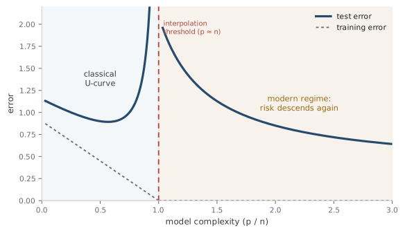
The regime past the peak is where the deepest surprise lives: benign overfitting, in which a model interpolates the training data — fits every point, noise included, to zero training error — and still predicts new data well. This directly contradicts the folk theorem that zero training error means memorization means poor generalization. Bartlett and coauthors made it precise for linear regression: they characterized exactly when the minimum-norm interpolator — the zero-training-error fit that is smallest in the ridge sense — has near-optimal risk, and showed it requires overparameterization of a specific kind, with the covariance spectrum having many small directions that harmlessly absorb the noise (Bartlett et al., 2020). Hastie and coauthors mapped the whole risk curve for ridgeless least squares in the proportional regime, confirming the second descent and showing that a vanishing ridge penalty can be optimal exactly where classical intuition says to regularize hard (Hastie et al., 2022).
A sharper question
If a model can interpolate pure noise and still generalize, is the bias–variance tradeoff simply wrong? No — it is incomplete, not false. The decomposition of risk into bias squared plus variance (Chapter 12) is an exact identity; nothing overturns it. What was wrong was the extra assumption that complexity, measured by raw parameter count, is what drives variance up. In the overparameterized regime, adding parameters can lower variance, because the minimum-norm solution spreads the noise across many nearly-flat directions where it does little damage, and the implicit regularization of choosing the smallest-norm interpolant behaves like a ridge penalty you never wrote down. Bias and variance still add up to the risk; the variance term just does not behave monotonically in the parameter count. The tradeoff is real — the U is genuinely there on the left — but the parameter count was never the right \(x\)-axis.
Common trap
Benign overfitting is not a license to interpolate noise and hope. It holds only under specific conditions on the covariance spectrum and the signal, and where those conditions fail, overfitting is as malignant as your instincts say. The honest reading is narrow: sometimes, with the right structure and enough overparameterization, interpolation is safe — not that regularization is obsolete. In most practical problems a well-tuned ridge or lasso still beats the interpolator, and knowing which regime you are in is itself an open, data-dependent question.
It is worth being clear-eyed about what is settled here and what is not, because this is the frontier and the theory is still being written. What is proven: the Marchenko–Pastur and Tracy–Widom laws for sample-covariance spectra; the minimax-optimal sparse rates for the lasso under restricted eigenvalue conditions; sharp risk formulas for linear and ridge regression in the proportional regime; and precise conditions for benign overfitting in linear models. What is understood but narrower than the headlines suggest: double descent is real and reproducible, but "overparameterization is good" is a statement about specific model classes and data distributions, not a universal law. What is open: how far these linear-model results extend to deep networks trained by gradient descent, where the effective model class is shaped by the optimizer as much as the architecture and no one yet has a clean risk formula; why real networks land in benign rather than malignant regimes; and how to do valid inference — honest confidence intervals, not just point prediction — in high dimensions, an active and unfinished program. The last frontier of this book is a frontier in the literal sense: past it, the map runs out.
Note
A caution about the word "modern." Double descent was not conjured from nothing in 2019 — statisticians had noticed non-monotone test-error curves and the strange competence of interpolation decades earlier, and part of what the recent wave did was give the phenomenon a name, a clean linear-model theory, and a reason to take it seriously. The lesson is one this whole book has repeated: a surprising empirical result is a prompt to find the assumption that failed, not a reason to throw out the theory. Here the failed assumption was "more parameters means more variance," and locating it precisely is what turned a paradox back into statistics.
And that is the through-line, now complete. The book began with distributions as the language for uncertainty (Part I), turned them into estimators and asked what makes one good (Part II, Chapter 6), graded estimators by their risk and confronted the fact that unbiased is rarely optimal (Part III), discovered in the shrinkage surprise that deliberately biasing an estimate can dominate the honest one (Part IV), built the machinery of testing and inference on top (Part V), and finally, in the asymptotics of Part VI, watched the fixed-\(p\) guarantees that justified everything give way in the high-dimensional regime where modern data actually lives. Each part answered the previous one's leftover question. The recurring moral — accept a little bias to buy a large cut in variance; judge a procedure by its risk, not its unbiasedness; be honest about where a method works and where it breaks — is not a collection of tricks but a single habit of thought. Theoretical statistics is not a bag of tests to memorize; it is the disciplined study of how to learn from data under uncertainty, and of how to know when you have learned something real. The frontier is open, the questions are live, and you now have the map. Go read the field's next chapter — or write it.
References
- Bartlett, P. L., Long, P. M., Lugosi, G., & Tsigler, A. (2020). Benign Overfitting in Linear Regression. Proceedings of the National Academy of Sciences. arXiv:1906.11300.
- Belkin, M., Hsu, D., Ma, S., & Mandal, S. (2019). Reconciling Modern Machine-Learning Practice and the Classical Bias–Variance Trade-Off. Proceedings of the National Academy of Sciences. arXiv:1812.11118.
- Bickel, P. J., Ritov, Y., & Tsybakov, A. B. (2009). Simultaneous Analysis of Lasso and Dantzig Selector. The Annals of Statistics. arXiv:0801.1095.
- Hastie, T., Montanari, A., Rosset, S., & Tibshirani, R. J. (2022). Surprises in High-Dimensional Ridgeless Least Squares Interpolation. The Annals of Statistics. arXiv:1903.08560.
- Johnstone, I. M. (2001). On the Distribution of the Largest Eigenvalue in Principal Components Analysis. The Annals of Statistics.
- Marchenko, V. A., & Pastur, L. A. (1967). Distribution of Eigenvalues for Some Sets of Random Matrices. Mathematics of the USSR-Sbornik.
- Stein, C. (1956). Inadmissibility of the Usual Estimator for the Mean of a Multivariate Normal Distribution. Proc. Third Berkeley Symposium on Mathematical Statistics and Probability.
Check yourself
A few questions to test the ideas from this chapter. Pick an answer to see whether it holds up.
-
You draw n samples of a p-dimensional standard Gaussian, whose true covariance is the identity, and compute the sample covariance matrix in the regime p/n approaching 0.5. What happens to its eigenvalues?
Entrywise consistency does not imply spectral consistency. Each entry of the sample covariance converges, but the eigenvalues are extreme summaries of the whole matrix, and small correlated errors across many entries push the top eigenvalue up and the bottom one down. The limiting spread is exactly the Marchenko–Pastur law; the largest eigenvalue's fluctuations follow the non-Gaussian Tracy–Widom law. There is no splitting into clusters and no shrinking to 1 — the spread persists no matter how much data of the same shape you collect. -
In p = 1000 dimensions, where does essentially all the probability mass of a standard Gaussian sit?
The density is indeed highest at the origin, but in high dimensions almost no volume is there — volume crowds toward the surface of the ball. The product of a low per-point density and an enormous volume peaks in a thin shell at radius root-p, with relative width shrinking as p grows. This is concentration of measure, and it is the engine of the curse of dimensionality: distances between points all concentrate near a single value, so nearness stops carrying information. -
The lasso attains estimation error of order root of (s log p over n) for an s-sparse signal, rather than root of (p over n). Which two facts make this rate possible?
The log p factor is the price of implicitly searching over all subsets of possible supports, since log of (p choose s) is about s log p. But sparsity alone is not enough: the restricted eigenvalue condition guarantees the true sparse signal is not confusable with a dense combination of the other predictors. Without it, two different sparse models can fit the data equally well and no method can separate them, so the rate is a property of the lasso on a recoverable design, not of the lasso alone. Knowing the support in advance would trivialize the problem — the whole point is that you do not. -
Double descent shows test error falling again in the overparameterized regime, sometimes below the classical sweet spot. What does this establish about the bias–variance decomposition?
Risk equals bias squared plus variance is an exact identity and nothing overturns it. The mistaken extra assumption was that raw parameter count drives variance up. In the overparameterized regime the minimum-norm interpolator spreads noise across many nearly flat directions where it does little harm, and choosing the smallest-norm fit acts like a ridge penalty no one wrote down. Bias and variance still sum to the risk; the variance term simply is not monotone in the parameter count, so the count was never the right complexity axis. -
A colleague concludes from benign overfitting that fitting the training data to zero error is always safe as long as the model is large enough. Where does this reasoning go wrong?
Bartlett and coauthors proved benign overfitting for linear regression only under conditions on the effective rank of the data covariance — many small directions to harmlessly absorb the noise. Outside those conditions, interpolation is as malignant as intuition says. In most practical problems a well-tuned ridge or lasso still beats the interpolator, and diagnosing which regime you are in is itself an open, data-dependent question. The result narrows to sometimes-safe, never to regularization-is-obsolete.