1What This Book Is About
You flip a coin a hundred times and it comes up heads fifty-three. Is the coin fair? You cannot know. A fair coin easily gives fifty-three; a slightly bent one gives fifty-three just as happily. The data you hold is a single roll of a die that may or may not be loaded, and you still have to say something. Theoretical statistics is the study of how to say that something well — and, the part that catches people off guard, how to grade your own method before you have seen a single number.
If you take one idea from this chapter, take this: statistics is one question wearing many costumes — how to turn uncertain data into a belief or a decision, and how to judge the rule you used before the data ever arrives.
The rest of the book is that question, followed patiently through six acts. This chapter draws the map so the acts feel like one argument rather than a drawer full of unrelated tools. There will be almost no formulas here; the point is to see the shape of the thing before we start measuring it.
1.1One question in many disguises
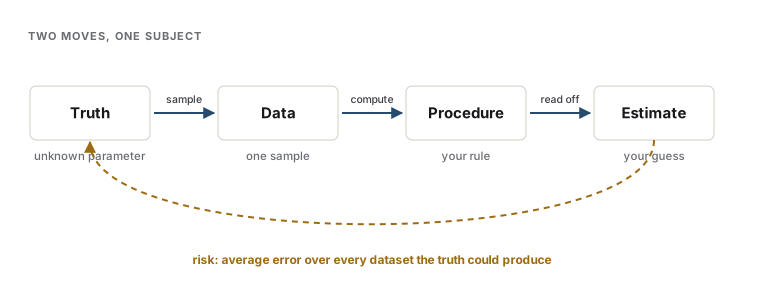
Everything begins with a gap between what you want to know and what you can see. What you want to know is a fixed feature of the world: the true bias of the coin, the average effect of a drug, the slope relating dose to response. Call such an unknown a parameter — a number (or a handful of numbers) that pins down which situation you are actually in. What you can see is data: a finite, noisy sample that the parameter helped produce but does not reveal directly.
To reason about that gap at all, you have to say how the data was produced. That declaration is a statistical model: a family of probability distributions, one for each possible value of the parameter, that you are willing to treat as the menu the world chose from. "The hundred flips are independent, each heads with probability \(\theta\)" is a model, and \(\theta\) is its parameter. The model is an assumption, not a fact — the whole craft lives in choosing one honest enough to be useful and simple enough to reason about.
Once you have a model, the first move is the obvious one: run the data through some rule to produce a guess. A rule that turns data into a guess for a parameter is an estimator, and choosing good ones is the business of Part II. But there is a second move, less obvious and more powerful, and it is what makes this a theory rather than a bag of recipes. Because the data is random, your guess is random too: rerun the world, draw a fresh sample, and the rule spits out a different number. The spread of answers a rule would give across all the samples the truth could have produced is its sampling distribution, and it is the object statistics actually reasons about. You judge a rule not by the one answer it gave you but by how it behaves over that whole cloud of might-have-been answers — how far off it lands on average, how much it jitters. That judgment can be made before you collect any data at all.
Intuition
Doing statistics is inference; the theory of statistics is judging the inference machine. You can score a rule the way you would score a factory — not by inspecting one item it made, but by the distribution of items it makes across every run.
A sharper question
If the parameter is a fixed number and the data is what actually happened, why reason about samples that never occurred? Because the quality of a rule is not a property of one dataset — it is a property of the rule. "This estimate equals 53" tells you nothing about whether the method was any good; a broken clock also produces a number. Only by asking what the rule would do across the samples the model allows can you say it is accurate, or precise, or trustworthy. The counterfactual samples are where all the guarantees live. This frequentist reading of "how good" is one of two great stances on that question; the Bayesian alternative, which treats the parameter itself as uncertain and updates belief with data, waits in Chapter 9.
1.2The map of the field
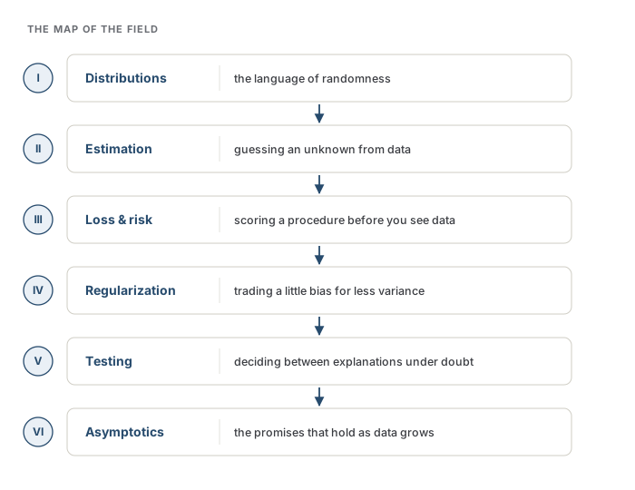
The subject is usually taught as a parade of techniques — the t-test, maximum likelihood, ridge regression, the bootstrap — and the parade hides that they are answers to one steadily deepening question. Read in order, the six parts of this book are a single chain, each link forced by the one before it.
You start with the language. Before you can say anything about data under uncertainty, you need a way to describe uncertainty itself, and that language is distributions: how a random quantity spreads its weight, how several such quantities interact, and what happens to their averages as data piles up (Part I, Chapters 2 through 5). With the language in hand, you can pose the first real task — estimation: given data from a model, produce a good guess for its parameter, and understand what "good" even means (Part II).
But "good" cannot be settled inside estimation. To compare two guesses you need a way to score being wrong, and that forces the next link: a loss function, a rule that says how much a given error costs, and its expectation over the sampling distribution, the risk (Part III). Risk is the scoreboard the whole field plays on. And the moment you have that scoreboard, a surprise falls out of it — the estimator that is right on average is usually not the one with the lowest risk. Deliberately biasing a guess, pulling it toward a sensible center, can lower its total error. That is regularization, and it is the argument of Part IV; the bias–variance tradeoff behind it is Chapter 12, and the paradox that makes shrinkage feel like a magic trick is Chapter 13.
Two acts remain, and they are the same ideas turned toward different jobs. Testing asks not "what is the parameter?" but "which of two stories does the data favor, and how sure can I be?" — decision-making under doubt, with its own accounting of the two ways to be wrong (Part V). And asymptotics cashes in a promise that has been hovering the whole time: as the sample grows, the messy small-sample picture collapses into a clean limiting one, which is why maximum likelihood is hard to beat and why the normal distribution keeps appearing (Part VI). The book ends where the theory is still being written, in high dimensions, where the classical intuitions bend.
Analogy
Distributions are the grammar, estimation is writing a sentence, and loss and risk are the editor who tells you whether the sentence is any good. Regularization is learning that the crispest sentence is often not the literal one, and testing is deciding which of two readings the evidence supports. The analogy leaks where every analogy to language leaks: grammar is a human convention you may bend for style, while a probability model is a claim about the world that is either adequate or not — and when it is wrong, no amount of elegant estimation on top of it can save you.
Note
The chain is the logical order, not a rule about what you may learn first. Bayesians, for instance, fold estimation, testing, and regularization into a single act of updating belief, and the loss function moves to center stage in a different way. The map is one honest route through the country, chosen so each idea arrives already motivated; it is not the only road.
1.3Why learn the theory, not the recipes
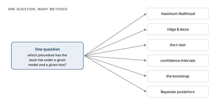
You could, in principle, skip all of this and memorize a decision tree: two groups and normal-looking data, run a t-test; too many predictors, run the lasso; want a standard error you cannot compute, run the bootstrap. The recipes work, and for the situations they were built for, they are exactly right. The trouble is that data does not arrive labeled with which recipe made it, and the interesting problems are precisely the ones no card in the box quite fits.
Theory is what you fall back on when the recipe runs out. It does two things a lookup table cannot. First, it tells you when a method works and when it fails — the t-test's promise leans on assumptions that a theory makes explicit and checkable, so you know the difference between using it and abusing it. Second, and more deeply, it lets you build the method you need when none exists, because every recipe in the box is the same underlying question — which procedure has the lowest risk under my model and my loss? — answered for one particular model and one particular loss. Maximum likelihood, ridge and lasso, confidence intervals, the bootstrap, the Bayesian posterior: these are not separate inventions but that one question solved under different assumptions. Learn the question, and the recipes stop being things to memorize and start being things you could have derived.
Common trap
The most common way to misuse statistics is to treat it as that decision tree — to match your situation to the nearest named test and read off a verdict, without ever checking whether the model the test assumes describes your data. A p-value computed under a false model is a precise answer to a question you did not ask. The recipes are safe only inside the assumptions the theory makes visible; skip the theory and you cannot see the fence you are standing outside of.
A sharper question
If it all reduces to "minimize risk," why is the book six parts long instead of one sentence? Because almost everything hard is hidden in the words "under my model and my loss." You rarely know the true model, the risk you care about is rarely the one that is easy to compute, and the estimator with the lowest risk is often impossible to write down and must be approximated. The unifying question is genuinely unifying — but each part of the book is a different piece of what it takes to answer it honestly on real data. That the pieces cohere is the reason to learn them together (Wasserman, 2004; Cox, 2006).
The map is drawn; the rest of the book walks it. We begin where every argument about uncertainty has to begin — with the language of distributions, in Chapter 2 (Hastie et al., 2009).
References
- Cox, D. R. (2006). Principles of Statistical Inference. Cambridge University Press.
- Hastie, T., Tibshirani, R., & Friedman, J. (2009). The Elements of Statistical Learning: Data Mining, Inference, and Prediction. Springer.
- Wasserman, L. (2004). All of Statistics: A Concise Course in Statistical Inference. Springer.
Check yourself
A few questions to test the ideas from this chapter. Pick an answer to see whether it holds up.
-
The chapter calls theoretical statistics 'one question in many disguises.' Which pairing best captures the two moves it says the subject is built from?
The first move is inference (data to a guess); the second, and the one that makes it a theory, is evaluating the procedure over its sampling distribution — before the data arrives. Testing and significance are one application, not the whole subject, and the second move is about grading the rule, not the single estimate it happened to output. -
Why does the book insist on reasoning about samples that never actually occurred?
'This estimate equals 53' says nothing about whether the method is good — a broken clock also emits a number. Guarantees like accuracy and precision live in what the rule would do across the samples the model allows. In the frequentist reading the parameter is fixed, not random; treating it as random is the Bayesian stance, a different framing. -
The chapter frames the six parts as a single chain in which each link is forced by the previous one. What forces the move from estimation to loss and risk?
'Good' cannot be settled inside estimation: comparing guesses requires a loss function and its expectation, the risk. That scoreboard is also what later reveals the bias-variance surprise. Risk is not a patch applied after estimating, nor a large-sample replacement for it — it is the yardstick that makes 'better' meaningful. -
A statistical model, as the chapter defines it, is best described as which of the following?
A model is a whole family of candidate distributions indexed by the parameter — a menu the world is assumed to have chosen from, not a proven fact. It is an assumption you adopt, distinct from the estimator that maps data to a guess; and adopting it guarantees nothing about whether it is adequate, which is exactly why checking it matters. -
The chapter argues you should learn the theory rather than memorize a table of named tests. What is the deeper of the two reasons it gives?
Beyond telling you when a method is valid (the first reason), the theory reveals that maximum likelihood, ridge, the bootstrap, and the rest are one question — least risk under a model and loss — solved under different assumptions, so you can build the method you need. It does not make assumptions disappear; it makes them visible, which is what keeps you from misusing a recipe.