15Choosing the Penalty
The penalty \(\lambda\) from the last chapter is a knob, and this chapter is about which way to turn it. Turn it to zero and you fit the data as hard as you can — all variance, an overfit model that has memorized the noise. Turn it up and you crush the coefficients toward zero — all bias, an underfit model too stiff to see the signal. Somewhere between sits the setting that minimizes prediction error, the bottom of the bias-variance U from Chapter 12. The trouble is that you cannot find it by looking at how well you fit the data you trained on, because that number always votes for \(\lambda = 0\). You need an honest estimate of how the model does on data it has not seen, and a way to read \(\lambda\) as an amount of complexity rather than a bare number.
If you take one idea from this chapter, take this: choosing the penalty is choosing model complexity, and cross-validation is how you let the data choose it honestly.
15.1Letting the data choose
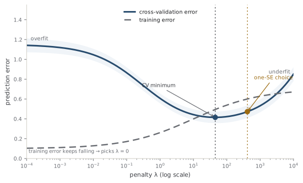
Start with the temptation and why it fails. You have a family of fits, one per value of \(\lambda\), and you want the best one. The obvious score is training error — the average loss on the very data you fit — so why not pick the \(\lambda\) that minimizes it? Because training error is not a measure of how good the model is; it is a measure of how hard the model tried. A model fit with \(\lambda = 0\) bends all the way to the data, driving training error down toward zero, and every increase in \(\lambda\) only stiffens the fit and raises training error. Minimizing it therefore always lands on \(\lambda = 0\): the most overfit model in the family.
Common trap
You cannot choose \(\lambda\) on the training set. Training error slides down monotonically as you weaken the penalty, so it will always crown the least-regularized, most-overfit model. The quantity you actually care about — error on new data — first falls and then rises, and the gap between the two curves is exactly the overfitting the training score cannot see.
What you actually care about is generalization error: the loss you would incur on a fresh observation drawn from the same process. You do not have fresh observations to spare, so you manufacture them by hiding some of your data from the fit and scoring on the part you hid. That is cross-validation: a way to estimate out-of-sample error using only the sample you have. In \(k\)-fold cross-validation you split the data into \(k\) roughly equal folds, then for each fold in turn you train on the other \(k-1\) and score on the one you held out, and finally you average the \(k\) held-out scores. Every observation is predicted exactly once, by a model that never saw it.
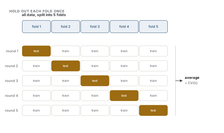
Run that whole procedure at each candidate \(\lambda\) and you trace out a curve. Write \(k(i)\) for the fold that holds observation \(i\), and \(\hat f^{-k(i)}_\lambda\) for the model fit at penalty \(\lambda\) on all folds except that one. The cross-validation error is the average held-out loss:
Plotted against \(\lambda\) this is a U (or a hockey-stick when the noise is mild): high on the left where the unpenalized fit overfits, high on the right where the heavy penalty underfits, with a dip in between. Pick the \(\lambda\) at the bottom and you have let the data tell you how much to shrink.
Intuition
Training error asks "how well did I fit what I have already seen?" — and the answer improves the harder you fit, which is no test at all. Cross-validation asks "how well would I do on something I have not seen?", and that answer gets worse once you start fitting noise. Only the second question has a wrong answer, which is exactly why it can guide you.
The minimum is not the only sensible choice. The CV curve is itself estimated from a finite sample, so its exact location jitters; the folds disagree, and that disagreement has a size. The one-standard-error rule takes the standard error of the CV score across folds at the best \(\lambda\), then picks the largest \(\lambda\) — the simplest, most regularized model — whose CV error is still within one standard error of the minimum. You give up a hair of estimated accuracy for a simpler, more stable model, on the theory that differences smaller than the noise in the curve are not worth chasing (Hastie et al., 2009).
Analogy
Cross-validation is like grading a student on held-back exam questions instead of the practice set they studied from. Score them on the practice problems and a memorizer looks brilliant; score them on questions they have not seen and you learn whether they understood anything. The analogy leaks in that exam questions are genuinely independent, whereas your folds are carved from one dataset and share its quirks — which is why CV estimates generalization error rather than measuring it exactly.
Common trap
If you tune \(\lambda\) by cross-validation, the tuned model must still be judged on data used nowhere in the tuning. The moment you pick \(\lambda\) by its CV score, that score stops being an unbiased estimate of error — you optimized against it, so it is optimistic. Any preprocessing that peeks at the whole dataset (standardizing features, selecting variables) has to happen inside each fold, not before the split; doing it once up front leaks the held-out data into the fit and quietly inflates your results. Keep a final test set the tuning never touches.
A sharper question
Why not just use leave-one-out — set \(k = n\), holding out a single point each time — so the training sets are as large as possible? Leave-one-out nearly eliminates the bias from training on less than the full data, but its folds are almost identical to each other, so their scores are highly correlated and the variance of the average can be large. It is also \(n\) times the compute unless a shortcut exists — and for linear smoothers one does, since leave-one-out error has a closed form in terms of the diagonal of the hat matrix you will meet in the next section. Five- or ten-fold CV is the usual compromise: enough training data to keep bias small, folds different enough to keep variance in check.
15.2Complexity as a dial
Cross-validation tells you which \(\lambda\) to use, but not what you bought with it. For that, translate the penalty into a complexity you can read off — and the surprise is that complexity need not be a whole number.
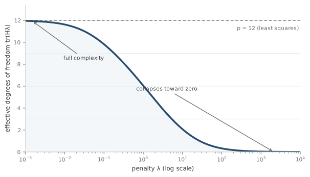
Without a penalty, a model's complexity is just its parameter count: fit \(p\) coefficients and you have spent \(p\) degrees of freedom, the number of independent directions in which the fit is free to chase the data. Regularization changes this. A penalized fit still has \(p\) coefficients, but it is not free to move each one as far as it likes — the penalty tethers them — so it behaves like a model with fewer parameters. The effective degrees of freedom make this precise: they measure how many parameters the fit effectively spends, and unlike a raw count they slide continuously.
The clean way to see it is through the hat matrix, the matrix \(H_\lambda\) that maps the observed responses to the fitted values, \(\hat y = H_\lambda y\) — so called because it "puts the hat on \(y\)." Its trace counts how sensitive the fitted values are to the observations, and that is the effective degrees of freedom. For ridge regression the trace has a beautiful closed form. Write the design matrix's singular values — the intrinsic scales of its directions — as \(d_1, \dots, d_p\). Then
Read the summand as a dimmer switch on each direction. When \(\lambda = 0\) every term is \(1\) and the sum is \(p\): full complexity, the ordinary least-squares fit. As \(\lambda \to \infty\) every term goes to \(0\) and so does the sum: the fit collapses to a constant, zero effective parameters. In between, a direction contributes near \(1\) when its scale \(d_j^2\) dwarfs the penalty (that direction is well-determined, so ridge leaves it alone) and near \(0\) when the penalty dwarfs it (that direction is shaky, so ridge all but discards it). The penalty spends your parameter budget preferentially on the directions the data actually pins down.
Intuition
Regularization does not turn parameters off one at a time; it turns them down. Effective degrees of freedom count the fractional total that survives — a model with \(p = 50\) nominal coefficients and a moderate penalty might have the complexity of, say, \(7.3\) genuine parameters. That fractional number, not the raw count, is what sits on the horizontal axis of the bias-variance U.
This is the payoff that ties the chapter together. The bias-variance curve of Chapter 12 has "model complexity" on its horizontal axis, and effective degrees of freedom are what that axis really means once you regularize. Sliding \(\lambda\) from \(\infty\) down to \(0\) walks the effective complexity from \(0\) up to \(p\), carrying you from the underfit right shoulder of the U, through its minimum, to the overfit left shoulder. Cross-validation, meanwhile, is estimating the height of that same U at each point. Choosing the penalty is choosing where on the complexity axis to stand, and the two tools work as a pair: effective degrees of freedom name the position, cross-validation tells you which position is lowest.
Note
Effective degrees of freedom generalize past ridge. Any linear smoother — a method whose fitted values are a fixed linear map of the responses, \(\hat y = Hy\) — has effective degrees of freedom \(\operatorname{tr}(H)\), which is why smoothing splines and \(k\)-nearest-neighbors can be placed on the same complexity axis and compared. The lasso is not a linear smoother, but a useful analogue holds: its effective degrees of freedom are well approximated by the number of nonzero coefficients it selects.
A sharper question
If cross-validation already scores every \(\lambda\), why bother computing effective degrees of freedom at all? Because CV gives you a black-box score with no interpretation — it says "this \(\lambda\) predicts best" without saying what kind of model that is. Effective degrees of freedom convert the penalty into a currency you understand and can compare across methods: a ridge fit with \(\text{df} = 7\) and a spline with \(\text{df} = 7\) are spending the same complexity, whatever their machinery. They also feed analytic model-selection criteria — AIC, generalized cross-validation — that estimate prediction error from the training fit plus a complexity charge of \(\text{df}(\lambda)\), giving you a cheaper, if more assumption-laden, alternative to running the folds. This complexity accounting becomes essential when \(p\) approaches or exceeds \(n\), the regime Chapter 21 takes up.
References
- Hastie, T., Tibshirani, R., & Friedman, J. (2009). The Elements of Statistical Learning: Data Mining, Inference, and Prediction. Springer.
Check yourself
A few questions to test the ideas from this chapter. Pick an answer to see whether it holds up.
-
Why can training error never be used to choose the penalty λ?
Weakening the penalty lets the fit bend harder toward the data, so training error only ever decreases as λ falls, bottoming out at λ = 0. It measures effort, not generalization. The gap between training error and held-out error is precisely the overfitting that training error cannot see. -
In k-fold cross-validation, what is each observation's contribution to CV(λ) computed from?
Each point is scored by the model trained on the other k-1 folds, so its prediction is genuinely out-of-sample. Rotating the held-out fold predicts every point exactly once. This is what makes CV(λ) an estimate of generalization error rather than a restatement of training error. -
For ridge regression, the effective degrees of freedom equal the sum over the design's singular values of d_j^2 / (d_j^2 + λ). As λ grows from 0 to infinity, this quantity does what?
Each term is a dimmer switch: near 1 when a direction's scale dwarfs λ, near 0 when λ dwarfs it. The sum starts at p (all terms 1) and decays smoothly to 0, so complexity becomes a continuous dial. Unlike the lasso, ridge never sets a coefficient exactly to zero; it fades them fractionally. -
What does the one-standard-error rule prescribe?
It steps toward more regularization: among all λ within one fold-to-fold standard error of the best CV score, choose the largest, giving the simplest model that is statistically indistinguishable from the best. The reasoning is that differences smaller than the curve's own noise are not worth chasing. -
You standardize all features and select variables using the full dataset, then run cross-validation to tune λ. What is wrong?
Any step that looks at the whole dataset before the split lets the held-out folds influence the fit, so the CV score is no longer an honest out-of-sample estimate. Preprocessing must happen inside each fold. And once λ itself is tuned by CV, that score is optimistic too, so a final untouched test set is needed to judge the tuned model. -
Compared with five- or ten-fold CV, what is the characteristic drawback of leave-one-out cross-validation?
Leave-one-out has low bias (training sets are nearly the full data) but its n folds overlap almost completely, so their scores are strongly correlated and the averaged estimate can have high variance. Five- or ten-fold CV trades a little bias for folds different enough to keep variance in check. For linear smoothers a closed form does exist, via the hat matrix diagonal.