4Families of Distributions

You have met a parade of named distributions by now — normal, Bernoulli, Poisson, exponential, gamma, beta — and it can feel like a zoo you are asked to memorize, each animal with its own formula, its own mean, its own quirks. The load-bearing surprise of this chapter is that most of them are the same animal wearing different coats. They share one algebraic skeleton, the exponential family, and once you can see it, three things that otherwise look like separate strokes of luck line up as one fact read three ways: the data has a natural summary you can keep and throw the rest away, a Bayesian prior updates without leaving its own family, and the mean drops out of a single derivative.

This is a "why does this keep appearing" chapter, not a catalog. The aim is to show you the shared form, watch a couple of familiar distributions fall into it, and then say plainly what the form buys — and, just as usefully, where it stops.

4.1One form behind many faces

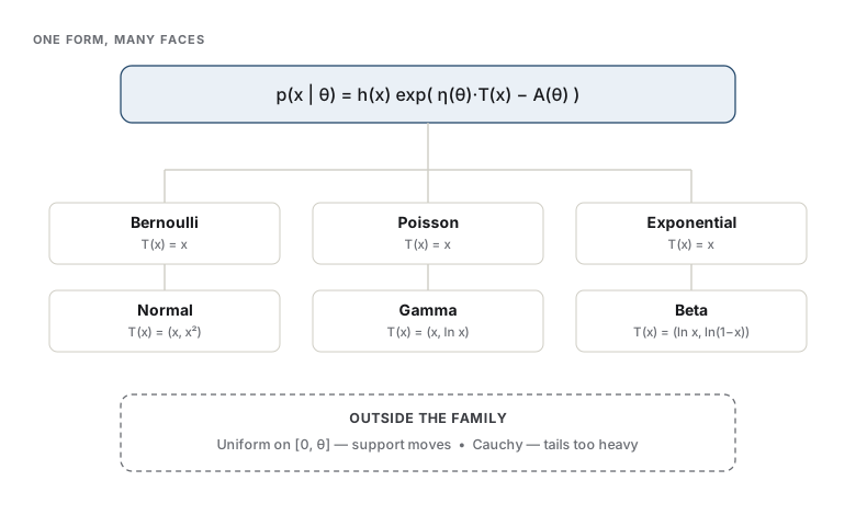
A family of distributions belongs to the exponential family if you can write its density (or, for discrete data, its mass function) in one particular shape. Introduced in words: the data \(x\) enters through a fixed summary, that summary is multiplied by a repackaged version of the parameter, the whole product sits inside a single exponential, and a normalizer out front keeps it a valid probability. Written out:

Read it one piece at a time, because every piece has a job:

• \(h(x)\) is the base measure — the part of the shape that does not move as \(\theta\) changes. It carries whatever is true of \(x\) regardless of the parameter (for counts, the \(1/x!\); for many families, just \(1\)).
• \(T(x)\) is the sufficient statistic — the only feature of \(x\) that the parameter ever touches. Everything the family cares about in a data point is squeezed into this one function.
• \(\eta(\theta)\) is the natural parameter — the parameter rewritten into the coordinate in which it multiplies \(T(x)\) linearly. This repackaging is the whole trick: in the right coordinate the parameter and the data meet in a plain dot product.
• \(A(\theta)\) is the log-partition function — the logarithm of whatever normalizing constant makes the density integrate to one, \(A(\theta) = \log \int h(x)\,e^{\eta(\theta)\cdot T(x)}\,dx\). It is fully determined by the other three pieces, and, as the next section shows, it quietly stores the family's moments.

The entire content of the definition is that last exponent: \(x\) shows up only through \(T(x)\), and it does so linearly in \(\eta\). Nothing else about \(x\) is allowed to interact with the parameter.

Make it concrete with the humblest distribution there is. A Bernoulli coin with success probability \(p\) has mass function \(p(x\mid p) = p^{x}(1-p)^{1-x}\) for \(x \in \{0,1\}\). Take the logarithm and regroup:

Line it up against the template: \(h(x)=1\), the sufficient statistic is \(T(x)=x\), the natural parameter is \(\eta = \log\frac{p}{1-p}\) — the log-odds — and \(A = -\log(1-p) = \log(1+e^{\eta})\). The natural coordinate of a coin flip turns out to be its log-odds, which is exactly the quantity logistic regression models linearly. The Poisson falls in the same way: \(p(x\mid\lambda)=\frac{\lambda^{x}e^{-\lambda}}{x!} = \frac{1}{x!}\exp(x\log\lambda - \lambda)\), so \(h(x)=1/x!\), \(T(x)=x\), \(\eta=\log\lambda\), and \(A=\lambda=e^{\eta}\).

4.2What the structure buys you

The form is not bookkeeping for its own sake. Three of the most useful facts in the subject fall straight out of it, and each is a preview of a chapter to come.

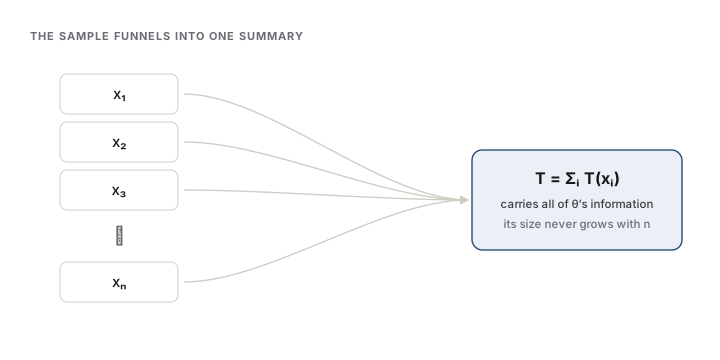
A sufficient statistic falls out for free. Suppose you draw an independent, identically distributed sample \(x_1,\dots,x_n\) from an exponential family. Multiply the densities and the exponents simply add:

Stare at where \(\theta\) appears: only alongside the single quantity \(\sum_i T(x_i)\). Once you know that sum (and \(n\)), the parameter cannot tell your actual dataset apart from any other dataset with the same sum. That is what it means for a statistic to be sufficient — it carries everything the sample knows about \(\theta\), so you may keep it and discard the raw data with no loss. For a coin you keep the number of heads; for a Poisson stream, the grand total; the order and the individual values are irrelevant. And crucially, the summary's size does not grow with \(n\): a million coin flips still compress to one count. Chapter 7 makes sufficiency precise through the factorization theorem, and the exponential form is the cleanest place it ever appears — the factorization is already staring at you in the equation above.

Priors update without leaving the family. Turn to the Bayesian picture (Chapter 9), where you place a distribution on \(\theta\) before seeing data and update it after. For an exponential family there is a matched family of priors — the conjugate priors — engineered so the posterior lands right back in the same family; the update just adjusts a couple of numbers rather than reshaping the whole distribution (Diaconis & Ylvisaker, 1979). A Beta prior on a coin's \(p\), met with Bernoulli data, gives a Beta posterior: you add your heads and tails to the prior's two counts and you are done. A Gamma prior on a Poisson rate stays Gamma. This is not a coincidence you get to be grateful for distribution by distribution; it is a structural consequence of the linear-in-\(\eta\) exponent, which is why conjugacy and the exponential family are usually taught in the same breath.

Moments and the MLE come from differentiating \(A\). The log-partition function looks like dead weight, but its derivatives are the moments of \(T\). In the natural coordinate,

The mean of the sufficient statistic is one derivative of the normalizer, and its variance is the second — a duality between the log-partition function and the family's cumulants that organizes a surprising amount of modern inference (Wainwright & Jordan, 2008). It also hands you maximum likelihood almost for free (Chapter 8): differentiate the sample log-likelihood, set it to zero, and the equation you get is \(\mathbb{E}_\theta[T(X)] = \frac{1}{n}\sum_i T(x_i)\). The maximum-likelihood estimate is whatever parameter makes the model's average of \(T\) equal the data's average of \(T\). Fit becomes moment-matching, and it is the sufficient statistic that both sides are matching on.

4.3Where the family ends

The exponential form is a wide net, but it is not the whole ocean, and the two most instructive misses tell you exactly what the structure was buying. Both break a single-line summary of the family: the parameter must touch the data only through \(\eta\cdot T(x)\), on a support that does not itself depend on \(\theta\).

The first classic outsider is the uniform distribution on \([0,\theta]\), with density \(p(x\mid\theta)=\frac{1}{\theta}\mathbf{1}\{0\le x\le\theta\}\). The trouble is the indicator: the set where the density is positive slides as \(\theta\) moves. You cannot fold a moving support into the template, because \(h(x)\) is required to be a fixed function of \(x\) alone and \(A(\theta)\) a fixed function of \(\theta\) alone — neither can encode "positive only up to \(\theta\)." Whenever the support depends on the parameter, the family is not exponential, full stop. This is the single most common way a distribution that otherwise looks tame falls outside.

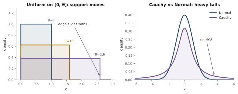
The second outsider keeps a fixed support but breaks the exponent a different way. The Cauchy distribution, \(p(x\mid\theta)=\frac{1}{\pi\,(1+(x-\theta)^{2})}\), is a location family on all of the real line, so its support is fixed — yet it is not exponential family. Its tails are too heavy: it has no moment-generating function and not even a finite mean, so the "differentiate \(A\) to get moments" machinery has nothing to grab. The practical shadow of this is stark. A Cauchy sample has no fixed-size sufficient statistic; to summarize where its center sits you essentially need the whole ordered sample, and the sample mean of Cauchy data is no more accurate than a single observation. Everything the previous section promised quietly fails, because the promise was made to the exponential family.

Seen this way, the exponential family is less a list to memorize than a explanation for why the list is short. The distributions you keep meeting are the ones that constrain a few averages and nothing more, and that single design decision is what makes them summarizable, updatable, and fittable at once. When you next meet a distribution that resists all three, check its support and check its tails — one of them will usually have stepped outside the form.

References

- Diaconis, P., & Ylvisaker, D. (1979). Conjugate Priors for Exponential Families. The Annals of Statistics.
- Wainwright, M. J., & Jordan, M. I. (2008). Graphical Models, Exponential Families, and Variational Inference. Foundations and Trends in Machine Learning.
Check yourself
A few questions to test the ideas from this chapter. Pick an answer to see whether it holds up.
-
What is the defining structural feature that makes a family of distributions an exponential family?
Exponential family is about algebraic form, not tail behavior: p(x | theta) = h(x) exp(eta(theta) . T(x) - A(theta)), with x entering only through T(x) linearly in eta. The tempting trap is to confuse the exponential *family* with the exponential *distribution* or with exponentially light tails, a different idea entirely; the Gaussian, Poisson, and beta are all in the family despite very different tails. -
You draw an independent, identically distributed sample of size n from an exponential family. What is enough to keep about the sample to lose nothing about theta?
Multiplying the densities makes the exponents add, so theta appears only alongside the single quantity sum of T(x_i): that sum (with n) is sufficient. Its dimension is fixed no matter how large n grows, which is the rare and precious property the exponential form guarantees. Keeping the sample mean and variance is only sufficient for special families such as the Gaussian, not in general. -
Why is the uniform distribution on [0, theta] not an exponential family?
The disqualifier is the moving support: 1{0 <= x <= theta} ties the positive region to theta, which the template forbids because h depends on x alone and A on theta alone. The 'no finite mean' option is a real fact about a *different* outsider, the Cauchy, planted here as a tempting cross-trap; the uniform has perfectly finite moments and still fails, for the support reason. -
The uniform on [0, theta] has the maximum of the sample as a one-dimensional sufficient statistic, yet it is not an exponential family. What does this establish?
Sufficiency alone is not the signature. The Pitman-Koopman-Darmois result gives exponential families a fixed-dimension sufficient statistic only *among families with fixed support*; drop that condition, as the uniform does, and you can still have a tidy sufficient statistic (the maximum) without being in the family. Fixed support is doing real work in the theorem. -
In the natural parameterization of an exponential family, how do you recover the mean of the sufficient statistic, E[T(X)]?
The log-partition function stores the cumulants: the first derivative of A gives E[T(X)] and the second gives Var(T(X)). That is why moments in an exponential family are a matter of differentiation rather than integration, and it is the same duality that powers modern variational inference. -
For an exponential family, the maximum-likelihood estimate of the parameter is characterized by which condition?
Setting the derivative of the log-likelihood to zero and using that A' = E_theta[T] turns fitting into moment-matching: pick the theta whose model average of T matches the data's average of T. The sufficient statistic is exactly the quantity both sides compare, tying maximum likelihood back to sufficiency.