13The Shrinkage Surprise
Here is a claim that sounds like a mistake. You want to estimate three unrelated numbers — a baseball player's batting average, the yield of a wheat field in Kansas, the price of a used car in Tokyo — and you have one noisy measurement of each. The obvious rule is to report each measurement as it stands: guess the batting average from the batting data, the yield from the yield data, and leave it there. Charles Stein proved in 1956 that this obvious rule is beatable. A single estimator that quietly pulls all three guesses toward a common number does better — not on average over some prior, but at every possible combination of the true values, with smaller total error, even though the three quantities have nothing to do with one another (Stein, 1956). This is Stein's paradox, and it is the reason the rest of Part IV exists.
If you take one idea from this chapter, take this: when you estimate three or more quantities at once, shrinking every estimate toward a shared center beats going it alone — because in many dimensions the raw estimates overshoot, and pulling them in cuts far more variance than the bias it adds.
13.1The estimator that should not exist
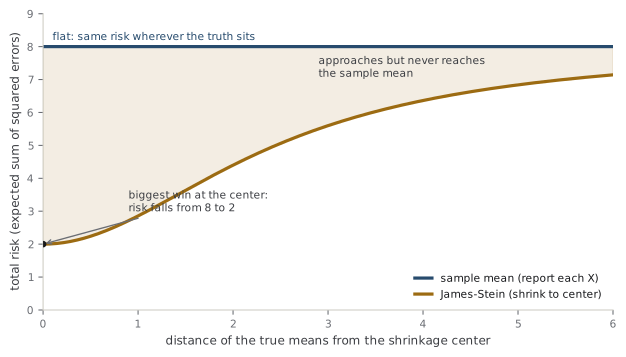
Set the problem up as cleanly as possible. You observe a vector \(X = (X_1, \dots, X_p)\), one noisy reading per unknown, where each \(X_i\) is centered on the truth \(\theta_i\) with variance \(\sigma^2\) and the readings are independent: \(X \sim \mathcal{N}(\theta, \sigma^2 I)\). You want the whole vector \(\theta\), and you grade yourself by total squared error, the sum over coordinates \(\sum_i (\hat\theta_i - \theta_i)^2\), whose expectation is the risk (Chapter 11). The natural estimator is the vector of sample means \(\hat\theta = X\) — coordinate by coordinate, it is unbiased, it is the maximum-likelihood estimate (Chapter 8), and in one dimension it is admissible and unimprovable (Chapter 11). Its risk is flat at \(p\sigma^2\): each coordinate contributes \(\sigma^2\), and they simply add.
Now the James-Stein estimator, the rule that shrinks. Pick a fixed center \(\nu\) to pull toward — for concreteness, the origin — and multiply the whole displacement \(X - \nu\) by a single data-dependent factor that is smaller when the readings sit close to the center and closer to one when they sprawl far from it:
Read the parenthesis as a dial between zero and one. When the readings cluster near \(\nu\), the squared distance \(\lVert X - \nu\rVert^2\) is small, the fraction is large, and the estimator pulls hard toward the center; when the readings are far-flung, the fraction shrinks toward zero and the estimator barely touches them. The astonishing fact, which James and Stein made precise in 1961, is that whenever \(p \ge 3\), this rule has strictly smaller risk than \(X\) at every single \(\theta\) (James & Stein, 1961). The plain sample mean is not just suboptimal; it is inadmissible (Chapter 11) — dominated everywhere by a rule that costs nothing extra to compute.
Intuition
You are not estimating one number; you are estimating a whole vector, and total error is what you pay. Shrinking each coordinate adds a little bias to that coordinate, but it strips a large, shared chunk of variance off the sum — and past three dimensions the variance you save always outweighs the bias you buy.
Note
The exact shrinkage factor is not magic tuning; the constant \(p-2\) is precisely what makes the risk calculation come out negative for every \(\theta\), and it is where the "three or more" threshold enters — at \(p = 2\) the factor gives no gain, and at \(p = 1\) it does not apply at all. A practical refinement, the positive-part James-Stein estimator, clips the factor at zero so the rule never flips a coordinate past the center; it dominates the raw version and is what you would actually use.
13.2Why the sample mean overshoots
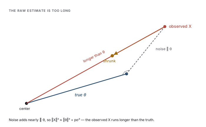
The dominance is real, so intuition owes you an explanation, and the honest one is geometric. In \(p\) dimensions the noise vector \(X - \theta\) has, on average, squared length \(p\sigma^2\) — one \(\sigma^2\) per coordinate. Crucially, in high dimensions that noise is almost perpendicular to the true vector \(\theta\): two generic directions in many dimensions are nearly orthogonal, so the noise adds to \(\theta\) at close to a right angle. Pythagoras then says the observed vector's squared length is about \(\lVert X \rVert^2 \approx \lVert \theta \rVert^2 + p\sigma^2\). The reading is systematically too long. Not sometimes — almost always, and by a predictable amount. So the vector \(X\) points roughly the right way but reaches past the truth, and pulling it back toward the origin moves it closer to \(\theta\).
Analogy
Imagine a swarm of arrows all fired at a target from the same spot, each blown off by an independent gust. In one or two dimensions the gusts scatter the arrows evenly around the bullseye. But add enough independent directions for the wind to blow in, and the arrows almost all land farther out than the bullseye, because there are vastly more ways to overshoot the center than to undershoot it. Reeling every arrow in by a common fraction brings the swarm closer. The analogy leaks in that real arrows do not know about each other, and neither does James-Stein — the pull is computed from the swarm's overall spread, not from any arrow's aim.
A sharper question
Why should shrinking help when the coordinates are genuinely unrelated — how can a batting average possibly borrow information from a wheat yield? It cannot, and it does not need to. The gain is not about the true values sharing structure; it is about the noise in your readings sharing a budget. Total variance is \(p\sigma^2\) no matter how the truths are arranged, and the overshoot \(\lVert X \rVert^2 \approx \lVert \theta \rVert^2 + p\sigma^2\) holds whatever \(\theta\) is. Shrinking spends one number — the observed overall spread — to correct a length error that is present regardless of relationship. Unrelated coordinates make the result feel like a swindle, but the arithmetic never asked whether they were related (Efron & Morris, 1977).
13.3Borrowing strength, and the rest of Part IV
The name statisticians give the winning move is borrowing strength, also called partial pooling: instead of estimating each quantity in isolation, you let the ensemble of estimates inform each one by pulling them all toward a common center. The word "borrowing" is apt and slightly misleading at once. No coordinate learns anything about its own truth from the others — the batting average is still estimated from batting data. What the ensemble supplies is a better sense of scale: seeing where the whole cloud of readings sits tells you how much of each reading is likely overshoot, and that shared estimate of the noise is what every coordinate borrows.
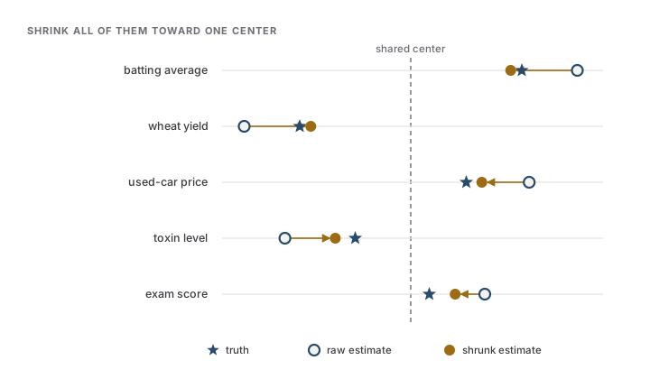
This is the deep reason regularization works, and it reframes everything that follows. Ridge regression, the lasso, a Bayesian prior, early stopping — the whole toolkit of Part IV is, at bottom, Stein's insight wearing different clothes: accept a little bias, aimed toward a sensible center, and collect a disproportionate cut in variance. Chapter 14 shows that shrinking toward zero is exactly what a prior centered at zero does, making "borrow strength" and "assume a prior" two descriptions of one act. Chapter 15 turns to the only question Stein leaves open — how far to shrink — which cross-validation answers with the data itself. And Chapter 21 shows that when the number of parameters grows with the sample size, this stops being a clever trick and becomes the only way to estimate at all: in high dimensions, shrinkage is not optional (Hastie et al., 2009).
Common trap
James-Stein lowers the total risk summed over all coordinates — it promises nothing about any single one. An individual estimate can get strictly worse: shrink a coordinate whose truth genuinely sits far from the center, and you have pulled it away from its target to help the sum. If you care about one specific coordinate on its own terms, the guarantee does not cover you; the paradox is a statement about the ensemble, and reporting a shrunken single estimate as if it were individually optimal is a misuse of the result.
Note
The reaction to Stein's result was not polite acceptance. It genuinely offended a generation of statisticians, because it says the sample mean — the most trusted estimator in all of statistics, unbiased and efficient by every classical criterion — is inadmissible the moment you estimate three things at once. The lesson that survived the shock is calmer than the scandal: unbiasedness is not sacred, "estimate each thing separately" is not free, and pooling is not cheating. It is, in high dimensions, simply the better bet.
References
- Efron, B., & Morris, C. (1977). Stein's Paradox in Statistics. Scientific American.
- Hastie, T., Tibshirani, R., & Friedman, J. (2009). The Elements of Statistical Learning: Data Mining, Inference, and Prediction. Springer.
- James, W., & Stein, C. (1961). Estimation with Quadratic Loss. Proc. Fourth Berkeley Symposium on Mathematical Statistics and Probability.
- Stein, C. (1956). Inadmissibility of the Usual Estimator for the Mean of a Multivariate Normal Distribution. Proc. Third Berkeley Symposium on Mathematical Statistics and Probability.
Check yourself
A few questions to test the ideas from this chapter. Pick an answer to see whether it holds up.
-
Stein's paradox says the vector of sample means is inadmissible for estimating three or more means at once. What exactly does the James-Stein estimator improve on, and where?
The dominance is over total (summed) risk and holds at every theta, which is what makes the sample mean inadmissible. It is emphatically not a per-coordinate guarantee: a single coordinate can get worse. And the win exists everywhere, not only near the center, though it is largest there and shrinks toward zero as the truth moves far away. -
Why does shrinkage help even when the quantities being estimated are utterly unrelated, like a batting average and a wheat yield?
The improvement is about the noise budget, not shared structure among the truths. In p dimensions the observed vector overshoots in squared length by about p sigma-squared no matter what theta is, and shrinking corrects that length error. Independence and 'exchangeability' are red herrings: the result needs neither a relationship nor a common meaning among the coordinates. -
The James-Stein estimator carries the constant p minus 2 in its shrinkage factor. What is the significance of that particular constant?
The p minus 2 is what forces the risk difference to favor shrinkage at all theta, and it is where the 'three or more' threshold lives: at p equal to 2 the factor yields no gain, and at p equal to 1 it does not apply. It is not a free tuning knob, and it does not preserve per-coordinate unbiasedness, which shrinkage deliberately gives up. -
In high dimensions, why is the plain observed vector X almost always 'too long' relative to the true mean vector theta?
Two generic high-dimensional directions are nearly orthogonal, so the noise adds to theta at close to a right angle and the squared length picks up the noise's own squared length, about p sigma-squared. The sample mean is unbiased, and squared error does not reward large estimates; the overshoot is a geometric fact about lengths, not a bias. -
A colleague uses James-Stein to estimate 30 quantities, then reports the shrunken estimate of one particular quantity as if it were the best possible estimate of that quantity alone. What is the problem?
Total-risk dominance says nothing about any single coordinate; one can be pulled away from a genuinely far-from-center truth to help the sum. Dominance does not descend to each coordinate, no shared prior is required, and estimating the center from the data is standard and does not by itself void the result.