3Expectation, Moments, and Their Uses
A distribution is a whole cloud of possibilities, but most of the time you want to reason about it with a single number — its center, its spread, its lopsidedness. This chapter is about how to extract those numbers, starting with the most important one. Expectation is the probability-weighted average of a random variable: every possible value pulls on the answer in proportion to how likely it is. Almost everything else in the book — bias, variance, risk, the law of large numbers — is expectation wearing a different hat.
If you take one idea from this chapter, take this: expectation is a linear operator, and that linearity holds whether or not the pieces are independent. It is the quiet workhorse that makes hard problems fall apart into easy ones.
3.1Expectation, and the one property that runs everything
The expectation (or expected value, or mean) of a random variable \(X\) is what you get by averaging its values, each weighted by its probability. For a discrete variable it is a sum, and for a continuous one an integral, but it is the same idea both times:
where \(p\) is the mass function and \(f\) the density from Chapter 2. The name "expected value" is a little misleading — it need not be a value \(X\) ever takes. A fair die has \(\mathbb{E}[X] = 3.5\), which you will never roll. It is the long-run average, the number the sample mean settles toward as you collect more data (that convergence is the law of large numbers, Chapter 5).
Analogy
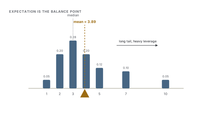
Think of the distribution as a set of weights placed along a rod, each value a position and each probability the mass sitting there. The expectation is the balance point — the spot where the rod would sit level on a fulcrum. This is exactly right, and it is why a long tail on one side drags the mean toward it. The analogy leaks in two places worth remembering: the balance point can sit where there is no mass at all (nothing lives at 3.5 on the die), and a rod with an infinitely heavy far tail has no balance point — a foreshadowing of the trap below.
The property that makes expectation indispensable is linearity. Scaling and shifting pass straight through, and — this is the surprising part — the expectation of a sum is the sum of the expectations, always:
Linearity of expectation asks nothing of \(X\) and \(Y\). They can be wildly dependent, even deterministic functions of each other, and the identity still holds exactly. This is what makes it a workhorse: to find the expected value of a complicated sum, you never have to understand how the pieces interact — you break the sum into parts, average each part alone, and add.
The classic demonstration is the hat-check problem. Handed back \(n\) hats at random, how many people expect to get their own? Let \(X_i\) be \(1\) if person \(i\) gets their own hat and \(0\) otherwise. These indicators are tangled together — if the first \(n-1\) people have their hats, the last one must too — so their joint behavior is a mess. But you never touch it. Each person has one chance in \(n\) of a match, so \(\mathbb{E}[X_i] = 1/n\), and
no matter how large \(n\) is. On average, exactly one person gets their hat. Computing this from the distribution of the total would be painful; linearity makes it a line.
Intuition
Expectation is an integral, and integrals are linear — they add up. Whether two quantities move together changes their joint distribution, but the expectation of each one alone reads only off its own margin, so summing expectations never asks the two margins to talk.
A sharper question
If dependence breaks the product rule — \(\mathbb{E}[XY] \neq \mathbb{E}[X]\,\mathbb{E}[Y]\) when \(X\) and \(Y\) are correlated — why does it spare the sum rule? Because the two rules read different things off the joint distribution. The expectation of a sum only needs each variable's marginal distribution, and the marginals are unaffected by how the variables are coupled. The expectation of a product genuinely probes the joint distribution — it asks how the two move together — so correlation shifts it. Independence is the extra ingredient that makes the product factor; the sum never needed it. This is why variance, which involves a square, is not linear across dependent variables, while the mean is.
Common trap
A distribution need not have a mean at all. The Cauchy distribution — the bell-shaped curve you get as the ratio of two independent standard normals — has tails so heavy that \(\int x\,f(x)\,dx\) does not converge, so \(\mathbb{E}[X]\) simply does not exist. This is not a technicality: sample means of Cauchy data never settle down, so the law of large numbers fails outright (Chapter 5). Before you write \(\mathbb{E}[X]\), you are quietly assuming the balance point exists. For heavy-tailed data it may not, and reaching for the mean anyway is a real mistake.
3.2Moments: the shape past the center
The mean locates a distribution but says nothing about its shape. To capture shape, you average not \(X\) but its powers — and those averages are the moments. The \(k\)-th moment is \(\mathbb{E}[X^k]\); more useful for shape are the central moments, which measure powers of the deviation from the mean, \(\mathbb{E}[(X - \mu)^k]\), where \(\mu = \mathbb{E}[X]\). Each higher power tells you something the lower ones cannot.
The second central moment is the variance (of a distribution), the average squared distance from the mean:
Its square root, the standard deviation, restores the original units and is the honest measure of spread. (This is the population version of the estimator variance from the bias–variance decomposition, Chapter 12 — same formula, applied to a distribution rather than to a \(\hat\theta\).) Squaring is what costs linearity: \(\operatorname{Var}(X+Y) = \operatorname{Var}(X) + \operatorname{Var}(Y)\) only when \(X\) and \(Y\) are uncorrelated, because the cross term \(2\,\mathbb{E}[(X-\mu_X)(Y-\mu_Y)]\) — the covariance — survives otherwise.
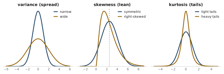
The third and fourth central moments, once standardized by dividing out the scale, name two features of shape you can see by eye. Skewness is the standardized third central moment; it measures asymmetry, and its sign tells you which tail is longer — positive for a long right tail, zero for anything symmetric. Kurtosis is the standardized fourth central moment; it measures how much of the variance comes from rare, extreme deviations, so it reads tail weight. The normal distribution has kurtosis \(3\), and people often subtract that off to define excess kurtosis, so that positive means heavier-tailed than a normal and negative means lighter.
Intuition
Read the moments in order as a zoom-out. The first fixes where the distribution sits, the second how wide, the third which way it leans, the fourth how fat its tails are. Each answers a question the previous ones left open.
Note
Moments do not always pin a distribution down. There are genuinely different distributions — the lognormal and certain perturbations of it are the standard example — that share every moment, all infinitely many, yet are not the same distribution. So knowing all the moments is not, in general, the same as knowing the law. This is the "moment problem," and it is exactly the gap the next section's tool closes when it exists.
3.3The moment generating function: a distribution's fingerprint
Instead of computing moments one at a time, you can pack all of them into a single function. The moment generating function (MGF) of \(X\) is the expected value of \(e^{tX}\), viewed as a function of the auxiliary variable \(t\):
The name is literal. Expand \(e^{tX}\) as its power series and take expectations term by term, and the moments fall out as the coefficients — equivalently, differentiate \(M_X\) at \(t = 0\) and the \(k\)-th derivative is the \(k\)-th moment, \(M_X^{(k)}(0) = \mathbb{E}[X^k]\). One function, differentiated repeatedly at the origin, generates the entire sequence of moments.
The MGF earns its keep through two properties. First, when it exists in an interval around \(t = 0\), it determines the distribution uniquely — no two different distributions share an MGF on such an interval. That makes it a fingerprint: recognize the MGF and you have identified the law, no matter how it was described to you. Second, and this is where it turns labor into arithmetic, the MGF of a sum of independent variables is the product of their MGFs:
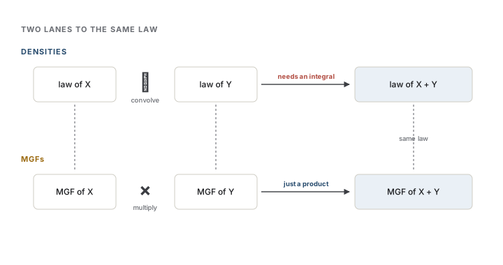
To see why the second property matters, recall what adding independent variables does to their densities: it convolves them, an integral that smears one distribution across the other. Convolutions are genuinely unpleasant to compute. The MGF converts that convolution into ordinary multiplication, so you can find the distribution of a sum by multiplying two functions and then recognizing the fingerprint of the result. This is how you prove, in a line each, that the sum of independent normals is normal, the sum of independent Poissons is Poisson, and the sum of independent gammas with a common rate is gamma: multiply the MGFs and read off the answer.
A sharper question
You keep saying "when it exists" — when doesn't it, and what do you do then? The MGF is an average of \(e^{tX}\), which explodes if the tails of \(X\) are heavy, so \(M_X(t)\) is finite near \(t = 0\) only when the tails decay at least exponentially. The Cauchy distribution from the last section has no MGF anywhere but at the origin; the lognormal has none for any positive \(t\). The fix is the characteristic function, \(\mathbb{E}[e^{itX}]\) with an imaginary exponent, which replaces the runaway \(e^{tX}\) with a bounded oscillation \(e^{itX}\) of magnitude one. It therefore exists for every distribution while keeping both magic properties — it uniquely determines the law and turns sums into products. The MGF is the friendlier tool when it exists; the characteristic function is the one that always does, and it is the machine behind the central limit theorem (Chapter 5).
Common trap
A finite mean and variance do not guarantee an MGF. A distribution can have every moment finite and still have no moment generating function — the lognormal is the standard cautionary case, since its moments grow fast enough that the series defining \(M_X(t)\) diverges for all \(t > 0\). "Has all its moments" is strictly weaker than "has an MGF," which is why the uniqueness guarantee is stated for the MGF (or characteristic function), not for the moment sequence.
Expectation and its moments are the vocabulary the rest of the book speaks in. Estimators are judged by the mean and variance of their sampling distributions (Chapter 6), risk is an expectation of loss (Chapter 11), and the exponential family of Chapter 4 is organized precisely around the moment structure the MGF exposes. Learn to see a distribution through its first few moments, and you will have the summary that most of statistics actually operates on.
Check yourself
A few questions to test the ideas from this chapter. Pick an answer to see whether it holds up.
-
You want the expected value of X + Y, where X and Y are strongly correlated. What does linearity of expectation let you do?
Linearity of expectation asks nothing of the joint distribution — the expectation of a sum reads only off each variable's marginal, which dependence leaves untouched. The covariance correction belongs to the variance of a sum, not its mean; that is the one squaring makes sensitive to dependence. -
For a standard Cauchy distribution, how does the sample mean of a large dataset behave as the sample size grows?
The Cauchy's tails are heavy enough that the integral defining E[X] diverges, so no mean exists and the law of large numbers has no target — the sample mean of Cauchy data is itself Cauchy, no matter how large n is. Symmetry supplies a center of symmetry but not a finite expectation. -
Two distributions share the same mean and the same variance, but one has visibly heavier tails. Which moment first tells them apart?
Tail weight is the province of the fourth central moment; both distributions could be symmetric, so skewness may be zero for each and distinguish nothing. Variance is equal by assumption, and the mean says nothing about shape — reading moments in order zooms from location to spread to lean to tails. -
Why is the moment generating function the natural tool for finding the distribution of a sum of independent variables?
For independent variables M_{X+Y}(t) = M_X(t) M_Y(t), so the convolution that combines densities becomes ordinary multiplication. Because an MGF (where it exists) determines the law uniquely, you recognize the product as a known distribution's fingerprint and read off the answer. -
A distribution has finite moments of every order. Must it then have a moment generating function in an interval around zero?
Having every moment finite is strictly weaker than having an MGF: the MGF needs the whole moment series to sum, which demands roughly exponential tails, and the lognormal's moments grow too fast for that. This is why the uniqueness guarantee is stated for the MGF or characteristic function, not for the raw moment sequence. -
For which of these identities is independence (or at least zero correlation) genuinely required, rather than optional?
The variance of a sum carries a covariance cross term that vanishes only when the two are uncorrelated. The expectation identities hold unconditionally, which is exactly the asymmetry the chapter dwells on: the mean is linear across dependent variables, but the variance is not.