Chapter 7

7Sufficiency and Information

A sample of a thousand coin flips and the single number "537 heads" are, for the purpose of learning the coin's bias, the same object. Everything the thousand flips can tell you about the bias is already in that count; the order they came in, which particular flips were heads, all of it is noise you can throw away without losing a thing. This chapter is about two questions that fall out of taking that idea seriously. First, what can you throw away — which summary of the data keeps all the information about the parameter, so the rest is discardable? That is sufficiency. Second, how much information was there to keep in the first place, and what does that quantity buy you? That is Fisher information, and its payoff is a hard floor — the Cramér–Rao bound — on how precisely any estimator can ever pin the parameter down.

If you take one idea from this chapter, take this: the data speaks about a parameter only through a sufficient statistic, and the sharpness with which it speaks is a number — the information — that sets the best precision you can hope for.

7.1Sufficiency: what to keep

Fix a parameter $\theta$ you are trying to learn and a sample $x_1,\dots,x_n$ drawn under it. A statistic $T(x_1,\dots,x_n)$ — any function of the data, like the sum, the maximum, or the whole ordered list — is a sufficient statistic for $\theta$ if it carries everything the sample knows about $\theta$. Chapter 4 gave you the slogan; here is the precise sense of it. Once you are told the value of $T$, the conditional distribution of the raw data no longer depends on $\theta$ at all.

Sit with that, because it is the whole definition. Imagine two people. One sees the full sample; the other is told only $T = t$ and then simulates a fake sample consistent with that value. If $T$ is sufficient, the second person can draw their fake data from a distribution that does not involve $\theta$ — and their simulated sample is statistically indistinguishable from a real one. Whatever the parameter was doing to the data, it did entirely through $T$. So there is nothing left in the raw data, beyond $T$, that could help you estimate $\theta$: the leftover is pure noise, generated by a mechanism that never consulted the parameter.

Intuition

A sufficient statistic is a lossless summary for the parameter. Hand it to someone and they know exactly as much about $\theta$ as if you had handed them the entire dataset — the rest of the data is randomness you can regenerate without ever knowing the truth.

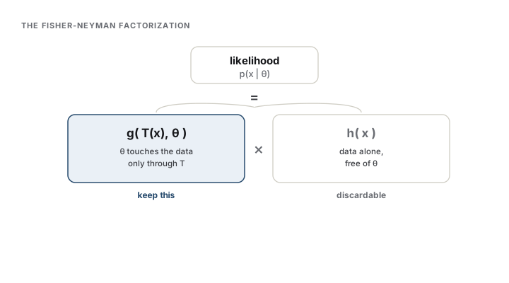
Checking sufficiency straight from that definition means computing a conditional distribution, which is miserable. The Fisher–Neyman factorization theorem replaces the whole exercise with a look at the shape of the likelihood. The likelihood is the sample's joint density read as a function of $\theta$ with the data held fixed — it scores how well each candidate $\theta$ explains what you saw. The theorem says: $T$ is sufficient for $\theta$ exactly when the likelihood factors into a piece that touches the data only through $T$ (and involves $\theta$), times a piece of the data alone (free of $\theta$):

\[p(x_1,\dots,x_n \mid \theta) = \underbrace{g\big(T(x),\,\theta\big)}_{\text{$\theta$ meets data only via } T} \;\cdot\; \underbrace{h(x)}_{\text{data alone, no } \theta}.\]

Read the split as a test you can actually run. Write down the likelihood, then try to quarantine $\theta$: if every appearance of the data that sits next to $\theta$ can be collected into a single function $T(x)$, that $T$ is sufficient. The factor $h(x)$ can be as ugly as it likes — it does not depend on $\theta$, so it scales every candidate parameter by the same amount and cannot change which $\theta$ the data prefers.

A diagram. A header box holds the likelihood p(x given theta). A downward split sends it into two boxes. The left box, tinted and outlined in the accent color, reads g(T(x), theta) and is labelled 'carries theta; touches the data only through T' with a note 'keep this'. The right box, plain, reads h(x) and is labelled 'data alone, no theta' with a note 'discardable for inference'. Below, a strip notes that because h(x) scales every theta equally, it cannot change which theta the data prefers. — Figure 7.1The factorization test made visual. The likelihood splits into a θ-bearing factor that sees the data only through T, and a θ-free factor of the raw data. Only the left box carries information about θ; the right one rescales every candidate parameter equally, so it drops out of any comparison.

The cleanest place this ever happens is the exponential family of Chapter 4, and you have already seen it. Write the joint density of an exponential-family sample and the exponents add: $$p(x_1,\dots,x_n\mid\theta) = \Big(\textstyle\prod_i h(x_i)\Big)\exp\!\Big(\eta(\theta)\cdot\textstyle\sum_i T(x_i) - nA(\theta)\Big).$$ The parameter $\eta(\theta)$ meets the data only alongside $\sum_i T(x_i)$, so that sum is the sufficient statistic — it falls straight out of the exponent, with the base-measure product $\prod_i h(x_i)$ playing the role of the $\theta$-free factor. For a coin you keep the head count; for a Poisson stream, the grand total. And crucially, this summary's size does not grow with $n$: a million flips still collapse to one count.

Analogy

Think of the likelihood as a recipe and $\theta$ as the one adjustable spice. Sufficiency asks: can you separate the recipe into "the part the spice touches" and "everything else"? If the spice enters only through, say, the total weight of the vegetables, then the total weight is all a taster needs to reverse-engineer how much spice you used. The analogy leaks where recipes are forgiving and likelihoods are not: the factorization must be exact, an algebraic identity, not an approximate separation — a whiff of $\theta$ left clinging to the discarded factor and $T$ is no longer sufficient.

A caution before leaving the idea. Many statistics can be sufficient at once, and some are wastefully large — the entire ordered sample is always sufficient, and useless as a summary because it throws nothing away. What you usually want is the smallest such summary, the minimal sufficient statistic: the coarsest function of the data that is still sufficient, the maximal compression you can perform without losing information about $\theta$. For the coin, the head count is minimal; you cannot compress further and still recover the likelihood's shape.

A sharper question

If I keep only $T$ and throw the rest away, have I not lost the ability to check whether my model was right in the first place? Yes — and this is the honest catch. Sufficiency is defined relative to a fixed model. The discarded factor $h(x)$ carries no information about $\theta$ assuming the model holds, but it is exactly where evidence of the model being wrong would live — a suspicious pattern in the order of the flips, say. So a sufficient statistic is the right thing to keep for estimating a parameter inside a model you trust, and the wrong thing to keep for criticizing the model. Goodness-of-fit checking lives in the residual you were told you could discard.

7.2Fisher information and the Cramér–Rao bound

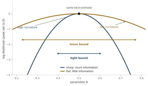
Sufficiency tells you what part of the data to keep. It says nothing about how much the kept part is worth — whether the sample pins $\theta$ down tightly or barely constrains it. That amount is a number, and the picture behind it is the single most useful image in this chapter: look at the log-likelihood as a function of $\theta$ and ask how sharply it peaks.

Recall the likelihood scores each candidate $\theta$ by how well it explains the data; take its logarithm and you get the log-likelihood, whose peak is the parameter the data most prefers (that peak is the maximum likelihood estimate of Chapter 8). Now compare two shapes of peak. A log-likelihood with a sharp, narrow peak says the data strongly distinguishes the best $\theta$ from its neighbors: move a little away from the top and the fit falls off a cliff. A flat, broad peak says the opposite — a wide range of $\theta$ explain the data almost equally well, so the data is barely committing to any of them. Sharpness is worth information; flatness is ignorance.

The quantity that measures sharpness is curvature. Define the score function as the slope of the log-likelihood in $\theta$, $\frac{\partial}{\partial\theta}\log p(x\mid\theta)$ — it is zero exactly at the peak. The Fisher information $I(\theta)$ is the expected squared score, which for smooth models equals the expected downward curvature at the truth:

\[I(\theta) = \mathbb{E}\!\left[\Big(\tfrac{\partial}{\partial\theta}\log p(X\mid\theta)\Big)^{\!2}\right] = -\,\mathbb{E}\!\left[\tfrac{\partial^2}{\partial\theta^2}\log p(X\mid\theta)\right].\]

The second form is the one to hold onto: information is the average curvature of the log-likelihood at the true parameter. Big curvature (a sharp peak) means big information; near-zero curvature (a flat peak) means almost none. And because a sample of $n$ independent draws adds $n$ log-likelihoods, their curvatures add too: total information is $nI(\theta)$, growing linearly with the sample size.

Intuition

Fisher information is the curvature of the log-likelihood at the truth. A sharp peak is a confident sample — small moves in $\theta$ are strongly penalized, so the data has a lot to say. A flat peak is a shrugging sample — many parameters fit about as well, so the data has little to say, no matter how many points you collected.

Here is the payoff. That curvature is not just a description of the data; it is a budget. The Cramér–Rao bound says that for any unbiased estimator $\hat\theta$ — one whose average over repeated samples lands exactly on $\theta$ — the variance cannot fall below the reciprocal of the total information:

\[\operatorname{Var}(\hat\theta) \;\ge\; \frac{1}{n\,I(\theta)}.\]

No cleverness gets you under this floor. A flat likelihood ($I$ small) forces a large minimum variance — the data simply cannot support a precise unbiased estimate. A sharp likelihood ($I$ large) permits a tiny one. The bound is the best precision the data can buy, set entirely by how sharply the model's likelihood responds to the parameter.

Figure 7.2Information is curvature. Two samples with the same best estimate: the sharp log-likelihood (high curvature) carries much information and permits a tight bound on any unbiased estimator; the flat one carries little and forces a loose bound. The width of the peak is, quite literally, the precision the data can afford.

An estimator that actually reaches the floor is called efficient, and its efficiency is the ratio of the bound to its variance — the fraction $\frac{1/(nI(\theta))}{\operatorname{Var}(\hat\theta)}$, which runs from $0$ (wasteful) up to $1$ (best possible). An efficient estimator wrings every drop of precision the data allows; an inefficient one leaves some on the table, achieving a variance larger than it had to. Efficiency is how you grade an estimator against the information floor rather than against other estimators.

Note

The bound reaches beyond one parameter. With several parameters at once, $I(\theta)$ becomes the Fisher information matrix — its entries are the expected curvatures and cross-curvatures of the log-likelihood surface — and the Cramér–Rao bound says the estimator's covariance matrix is at least the inverse of $nI(\theta)$. The one-dimensional story is the whole idea; the matrix just bookkeeps how information about one parameter can be spent, or lost, distinguishing it from another.

Common trap

The bound is a statement about unbiased estimators, and that qualifier is load-bearing. Biased estimators routinely beat it — the shrinkage estimators of Chapter 12 accept a little bias precisely to drop their variance below what any unbiased rule could reach. So "variance below $1/(nI)$" does not mean someone made an arithmetic error; it usually means they gave up unbiasedness on purpose. The Cramér–Rao floor is the price of insisting on being centered, not a universal speed limit on error.

A sharper question

If most sane estimators never reach the floor exactly, why is the bound worth anything? Because it becomes achievable in the limit. Under mild conditions the maximum likelihood estimator is asymptotically efficient: as $n$ grows its variance approaches $1/(nI(\theta))$, so the bound stops being a floor no one touches and becomes the exact large-sample variance of the estimator you were going to use anyway (Chapter 19). That is why Fisher information appears twice in this book — here as a hard limit, and later as the actual precision maximum likelihood delivers when the data is plentiful.

Seen together, the two halves of this chapter are the same statement read at two resolutions. Sufficiency identifies the channel through which the parameter speaks to the data; Fisher information measures the volume it speaks at; and the Cramér–Rao bound converts that volume into the best precision any honest, centered estimate can achieve. The next chapter takes the estimator that most fully exploits this structure — maximum likelihood — and asks why, and when, it works.

Check yourself

A few questions to test the ideas from this chapter. Pick an answer to see whether it holds up.

What is the precise sense in which a statistic T is sufficient for a parameter theta?
The Fisher-Neyman factorization writes the likelihood as g(T(x), theta) times h(x). Why can the factor h(x) be ignored when inferring theta?
Fisher information I(theta) is often described as the curvature of the log-likelihood at the truth. What does a small I(theta) tell you?
An estimator is reported with variance strictly below 1/(n I(theta)). What is the most likely explanation?
The maximum likelihood estimator usually does not attain the Cramer-Rao bound exactly at finite n. Why is the bound still central to how it is judged?
The entire ordered sample is always a sufficient statistic. What does this reveal about sufficiency?