AA Probability Refresher
This appendix collects, in one scannable place, exactly the probability the chapters lean on — the load-bearing definitions, identities, inequalities, and limit results, stated compactly and cross-referenced to the chapters that develop them. It assumes you have had a first probability course and that Part I has already built distributions, expectation, and the limit theorems in depth; nothing here re-teaches those, it reminds you of the facts and points back. Treat it as a cheat-sheet, not a chapter: each entry is the fact you reach for, with a pointer to where the reasoning lives.
A.1Distributions, conditioning, and independence
Probability begins with a sample space \(\Omega\) — the set of every outcome an experiment could produce — and events, the subsets of \(\Omega\) you can assign a probability to. A probability \(\mathbb{P}\) obeys the three probability axioms (Kolmogorov's): \(\mathbb{P}(A) \ge 0\) for every event, \(\mathbb{P}(\Omega) = 1\), and countable additivity — for disjoint events the probability of their union is the sum of their probabilities. Every rule below is derived from these three.
A random variable \(X\) is a number whose value is uncertain, formally a function from outcomes to the real line; its distribution says where its probability lives. That distribution has three interchangeable notations, developed fully in random variables and distributions, Chapter 2:
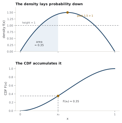
The cumulative distribution function (CDF) \(F\) always exists, runs from \(0\) to \(1\), and never decreases. The probability density function (pdf) \(f\) is its slope for a continuous \(X\), so probability over an interval is area, \(\mathbb{P}(a \le X \le b) = \int_a^b f\); the probability mass function (pmf) \(p\) is the direct probability of each value for a discrete \(X\). A density is a rate, not a probability: \(f(x)\) can exceed one, only the area is capped at one.
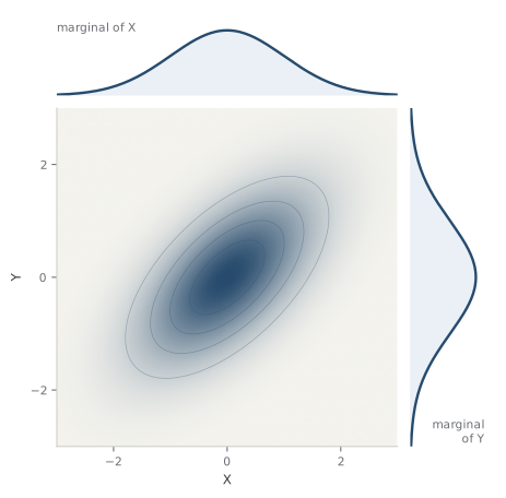
Track two variables at once and you need the joint distribution, which spends the unit of probability over pairs. From it you recover either variable alone by summing the other away (the marginal), or fix one and renormalize (the conditional):
The marginal is the joint's shadow on one axis; the conditional is a renormalized slice through it. Correlation lives only in the joint and is erased in either shadow — the marginals do not determine the joint.
Two variables are independent when knowing one tells you nothing about the other, which is exactly when every conditional equals the matching marginal and the joint factors:
Data assumed independent and identically distributed (i.i.d.) — mutually independent draws sharing one distribution — have a joint density that is the product of the individual densities, which is why the log-likelihood is a sum and the limit theorems fire (Chapter 2). Conditioning also runs the Bayesian engine through Bayes' rule, which reverses the direction of a conditional:
Common trap
Uncorrelated is weaker than independent. Zero covariance rules out only a linear relationship; independence rules out every dependence. Uncorrelated-but-dependent variables are easy to build (place mass symmetrically on a ring), so never read "uncorrelated" as "independent."
A.2Expectation, variance, and useful inequalities
The expectation \(\mathbb{E}[X]\) is the probability-weighted average of \(X\), the balance point of its distribution, developed with the moments in expectation, moments, and their uses, Chapter 3. Its workhorse property is linearity, which holds whether or not the variables are independent:
To average a function of \(X\) you do not need the distribution of that function — the law of the unconscious statistician (LOTUS) integrates \(g\) against the distribution you already have:
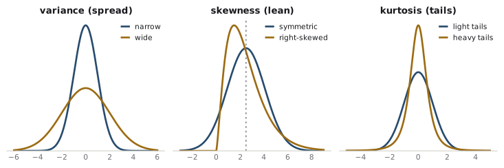
Variance measures spread, \(\operatorname{Var}(X) = \mathbb{E}[(X - \mu)^2] = \mathbb{E}[X^2] - \mu^2\), and covariance measures joint movement, \(\operatorname{Cov}(X, Y) = \mathbb{E}[(X - \mu_X)(Y - \mu_Y)]\). Variance is not linear: the cross term makes
so variances add only when the variables are uncorrelated. The moment generating function (MGF) \(M_X(t) = \mathbb{E}[e^{tX}]\) is a fingerprint: where it exists near zero it pins the distribution down uniquely, its derivatives at zero return the moments, and it turns sums of independent variables into products (Chapter 3).
Conditioning has an expectation of its own. The conditional expectation \(\mathbb{E}[Y \mid X]\) is the mean of \(Y\) within each slice \(X = x\), itself a random variable (a function of \(X\)). Averaging it back over \(X\) recovers the plain mean — the law of total expectation, or tower property — and the spread decomposes the same way, into within-slice and between-slice pieces, by the law of total variance:
Conditional expectation is also the object sufficiency is built on: conditioning on a sufficient statistic loses no information about the parameter (sufficiency and information, Chapter 7).
Three inequalities carry most of the weight in proofs. Jensen's inequality says a convex function and an average do not commute — the function of the mean sits below the mean of the function:
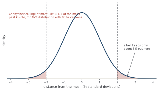
Markov's inequality bounds how much mass a nonnegative variable can push into its right tail, and squaring the deviation turns it into Chebyshev's inequality, a distribution-free bound on being far from the mean:
Intuition
Chebyshev converts a shrinking variance directly into a shrinking chance of being far off, with no distributional assumption at all. That is the whole mechanism behind the weak law of large numbers: drive \(\operatorname{Var}(\bar X_n) = \sigma^2/n\) to zero and the probability of straying from \(\mu\) is squeezed to zero with it.
A sharper question
If Chebyshev is so loose — 25% where the truth is 5% — why lean on it? Because it asks almost nothing in return: only a finite variance, no shape, no tail behavior, no independence. That universality is the point. When you know the distribution you can do far better (the central limit theorem gives the sharp normal tail), but when you know only that a variance exists, Chebyshev is often the only bound available, and it is enough to prove consistency.
A.3Convergence and the limit theorems
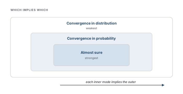
A sequence of random variables can approach a limit in several inequivalent senses, laid out in full in convergence and the limit theorems, Chapter 5. Four modes matter here. Convergence in probability (\(X_n \xrightarrow{p} X\)): for every tolerance \(\varepsilon > 0\), \(\mathbb{P}(|X_n - X| > \varepsilon) \to 0\). Almost sure convergence (\(X_n \xrightarrow{a.s.} X\)): the observed path itself converges, \(\mathbb{P}(\lim_n X_n = X) = 1\). Convergence in mean square: \(\mathbb{E}[(X_n - X)^2] \to 0\), a statement about the average squared gap. Convergence in distribution (\(X_n \xrightarrow{d} X\)): the CDFs converge, \(F_n(x) \to F(x)\) at every continuity point of \(F\) — a statement about shape, not location.
The modes are ordered, and the arrows run one way only:
Convergence in probability does not imply almost sure convergence, and convergence in distribution implies the rest only when the limit is a constant.
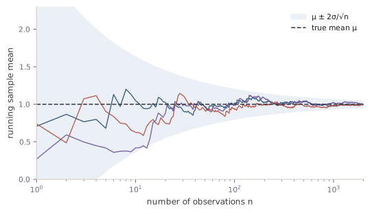
For an i.i.d. sample with mean \(\mu\) and finite variance \(\sigma^2\), the two limit theorems describe the sample mean \(\bar X_n\). The law of large numbers (LLN) says it settles on the truth, \(\bar X_n \xrightarrow{p} \mu\) (weak law) or \(\bar X_n \xrightarrow{a.s.} \mu\) (strong law). The central limit theorem (CLT) says how it fluctuates on the way, once magnified by \(\sqrt{n}\):
The source distribution vanishes from the right-hand side: only the mean and variance survive, which is why the spread \(\sigma/\sqrt{n}\) — the standard error — is the margin you attach to an average.
Two tools let you carry these limits through transformations. The continuous mapping theorem says a continuous \(g\) preserves convergence: if \(X_n \to X\) (in probability or in distribution), then \(g(X_n) \to g(X)\) in the same mode. Slutsky's theorem handles a converging-in-distribution term combined with one that converges to a constant: if \(X_n \xrightarrow{d} X\) and \(Y_n \xrightarrow{p} c\), then \(X_n + Y_n \xrightarrow{d} X + c\) and \(X_n Y_n \xrightarrow{d} cX\) (and \(X_n / Y_n \xrightarrow{d} X/c\) for \(c \ne 0\)). Slutsky is what lets you replace an unknown \(\sigma\) by a consistent estimate inside a CLT statement without disturbing the limit.
The delta method pushes the CLT through a smooth transformation. If \(\sqrt{n}\,(\hat\theta_n - \theta) \xrightarrow{d} \mathcal{N}(0, \sigma^2)\) and \(g\) is differentiable with \(g'(\theta) \ne 0\), then
The one-line idea: linearize \(g\) by its tangent at \(\theta\), so \(g(\hat\theta_n) - g(\theta) \approx g'(\theta)\,(\hat\theta_n - \theta)\), and a linear image of an asymptotically normal quantity is asymptotically normal with the slope squared into the variance. These three results are the machinery behind the asymptotic normality of estimators and their standard errors (asymptotic efficiency, Chapter 19), and behind the resampling approximations of the bootstrap, Chapter 20.
Intuition
The delta method is the CLT seen through a magnifying lens of curvature: near \(\theta\) the function \(g\) looks like its tangent line, and a straight-line transformation only rescales a bell by its slope. A steep \(g\) stretches the noise (a large \(g'(\theta)^2\)), a flat one compresses it, and a stationary point (\(g'(\theta) = 0\)) breaks the first-order method entirely.
Check yourself
A few questions to test the ideas from this chapter. Pick an answer to see whether it holds up.
-
For two random variables X and Y that may be dependent, which statement is correct?
Linearity of expectation is unconditional — it never needs independence. Variance is different: Var(X + Y) = Var(X) + Var(Y) + 2 Cov(X, Y), so variances add only when the covariance vanishes (uncorrelated is enough; full independence is not required). The two operations are often confused precisely because linearity is so forgiving. -
Among the modes of convergence, which implication is valid in general?
The arrows run one way: almost sure ⇒ in probability ⇒ in distribution, and mean square ⇒ in probability. The reverses fail — a sequence can converge in probability while its individual paths do not settle (almost sure fails), and convergence in distribution is only about the shape of the limiting law, so it implies the stronger modes only when the limit is a constant. -
If √n(θ̂ − θ) converges in distribution to Normal(0, σ²), what does the delta method give for a smooth g with g'(θ) ≠ 0?
Linearize g at θ: g(θ̂) − g(θ) ≈ g'(θ)(θ̂ − θ). A linear image of an asymptotically normal quantity is asymptotically normal, and scaling a random variable by a constant multiplies its variance by that constant squared — so the slope enters as g'(θ)², not to the first power and not the function's value. A stationary point g'(θ) = 0 kills the first-order term and the method must be taken to second order. -
Chebyshev's inequality bounds the mass beyond k standard deviations by 1/k², about 25% at k = 2, where a normal keeps only about 5%. Why lean on so loose a bound?
Chebyshev's power is its universality: a finite variance is the only assumption, so it holds distribution-free. That is exactly what makes it prove consistency — drive Var(X̄ₙ) = σ²/n to zero and the probability of straying from the mean is squeezed to zero with no shape assumption. When you do know the distribution, the CLT gives a far sharper normal tail; Chebyshev is the tool of last resort, not a tight one. -
What does the law of total expectation (the tower property) state?
The conditional expectation E[Y | X] is itself a random variable — a function of X — and averaging it over the distribution of X returns E[Y], for any X and Y. It is not restricted to the independent case (independence instead makes E[Y | X] = E[Y] the constant). The companion law of total variance splits Var(Y) into the mean of the within-slice variance plus the variance of the slice means. -
Jensen's inequality says that for a convex function g, how do g(E[X]) and E[g(X)] compare?
Convexity bends the curve upward, so chords lie above the graph and averaging inputs undershoots the averaged output: g(E[X]) ≤ E[g(X)]. Taking g(x) = x² recovers E[X²] ≥ (E[X])², which is just Var(X) ≥ 0. The inequality flips for concave g, and equals only for linear g or a degenerate X — expectation does not pass through nonlinear functions.