14Penalties and Priors
Fit a regression with more predictors than you can trust and the least-squares answer starts to thrash: tiny changes in the data swing the coefficients wildly, because the fit spends its freedom chasing noise. The cure from Chapter 12 is to add a penalty on how large the coefficients are allowed to grow — pay a price for magnitude, and the fit stops overreaching. This chapter is about the two penalties everyone reaches for first, ridge and lasso, why they behave so differently, and the quiet fact that adding a penalty is the same act as believing, before you saw any data, that the coefficients are probably small.
If you take one idea from this chapter, take this: a penalty on coefficient size and a prior belief that coefficients are small are the same statement in two languages — ridge is a Gaussian prior, lasso a Laplace one — so "shrink toward zero" and "expect near-zero" are one idea, not two.
14.1Ridge, lasso, and what they prefer
Start with ordinary least squares, which picks the coefficients \(\beta\) that minimize the residual sum of squares \(\sum_i (y_i - x_i^\top\beta)^2\) — the total squared miss over your \(n\) data points. Regularization (Chapter 12) adds a second term that grows with the size of \(\beta\), so the fit must now balance matching the data against keeping its coefficients small. The two famous choices differ only in how they measure size. Ridge regression (Hoerl & Kennard, 1970) penalizes the sum of squared coefficients — the squared L2 penalty, written \(\sum_j \beta_j^2\) — while the lasso (Tibshirani, 1996) penalizes the sum of absolute values — the L1 penalty, \(\sum_j |\beta_j|\):
The knob \(\lambda \ge 0\) sets the exchange rate between fit and size. At \(\lambda = 0\) both reduce to least squares; as \(\lambda \to \infty\) both crush every coefficient toward zero. That much they share. The difference is what happens in between, and it is stark: ridge slides every coefficient smoothly toward zero and keeps them all, while lasso drives some coefficients to exactly zero — it does not merely shrink the weak predictors, it deletes them. A fit with exact zeros is a sparse model, one that uses only a subset of the predictors, so lasso performs variable selection as a side effect of shrinking. Sparsity — most coefficients being exactly zero — is the property that makes lasso a model-selection tool and ridge merely a shrinkage tool.
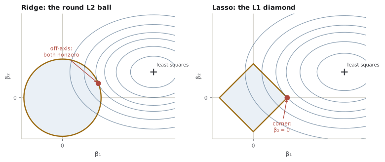
The cleanest way to see why comes from rewriting each fit as a budget problem. Minimizing residuals plus \(\lambda \times (\text{size})\) is equivalent to minimizing residuals alone subject to a hard cap on size: \(\sum_j \beta_j^2 \le t\) for ridge, \(\sum_j |\beta_j| \le t\) for lasso, with the budget \(t\) shrinking as \(\lambda\) grows. Now the geometry does the talking. The residual sum of squares, as a function of \(\beta\), has elliptical contours centered on the unconstrained least-squares solution; the fit you actually report is the point where the smallest such ellipse first touches the allowed region. For ridge that region is a round ball, and a ball has no special points — the ellipse can kiss it anywhere, almost surely off the axes, so every coefficient stays nonzero. For lasso the region is a diamond, and a diamond has corners that jut out exactly on the axes. An expanding ellipse tends to strike a corner first, and a corner is a coefficient set to zero.
Intuition
Squaring punishes a coefficient of 10 far more than ten coefficients of 1, so ridge spreads shrinkage thinly across everything; absolute value charges the same rate whether a coefficient is large or tiny, so lasso finds it worthwhile to zero out the small ones entirely.
Slide the penalty in the widget below and watch the two philosophies play out over the whole range of \(\lambda\). The dashed ridge paths ease every coefficient smoothly toward zero and arrive together only in the limit — no coefficient is ever exactly zero at a finite \(\lambda\). The solid lasso paths do something visibly different: each one travels down and then snaps to exactly zero at its own value of \(\lambda\), switching that variable off for good. Push \(\lambda\) up and the lasso model sheds predictors one by one until only the strongest survive, while the ridge model merely fades as a whole.
Analogy
Think of a fixed budget you must split across projects. Ridge is a manager who taxes every project in proportion to its size, so all survive on trimmed funding. Lasso is a manager who, facing the same squeeze, defunds the weakest projects completely to keep the strong ones healthy. The analogy leaks where budgets do not: real coefficients can be negative, and "size" for lasso means distance from zero in either direction, so a project can also be cut for being too far below the line.
Common trap
Lasso's exact zeros are seductive, and two misreadings follow. First, a coefficient the lasso sets to zero is not thereby proven to be "really" zero — the zero is manufactured by the diamond's corner, an artifact of the L1 geometry, not a discovery that the predictor has no effect. Second, when predictors are correlated the lasso becomes unstable: among a cluster of collinear variables it tends to keep one almost arbitrarily and zero the rest, and which one it keeps can flip with a slightly different sample. Read a lasso's selected set as one plausible sparse story, not as the truth about which variables matter.
A sharper question
If ridge never produces a zero, is it just a worse lasso whenever you want a simple model? No — they answer different questions. When the true signal is genuinely spread across many small effects, ridge usually predicts better, because forcing most coefficients to zero throws away real (if faint) structure. When the truth really is sparse, or you need an interpretable shortlist of predictors, lasso wins. And when predictors are correlated, ridge's habit of sharing weight across a cluster is a feature, not a bug — the very case where lasso's selection turns fragile. Choosing between them, and tuning \(\lambda\), is the subject of Chapter 15; the elastic net there splits the difference by summing both penalties.
14.2Regularization is a prior
Everything above was frequentist — a fit, a penalty, a knob. Yet the penalized objectives are identical to something from the Bayesian view of Chapter 9, and seeing the identity is the point of this chapter. Recall the maximum a posteriori (MAP) estimate: the value of \(\beta\) that maximizes the posterior, which by Bayes' rule is proportional to the likelihood times the prior distribution \(p(\beta)\). Maximizing the posterior is the same as maximizing its logarithm, and taking a logarithm turns the product into a sum. Flip the sign to turn the maximization into a minimization, and the MAP estimate reads
The first term is the negative log-likelihood — the fit. The second is the negative log-prior — the penalty. A penalized regression is nothing but a MAP estimate: the loss you minimize is the likelihood you assume, and the penalty you add is the prior you assume. Which prior gives which penalty is the beautiful part.
Take the standard regression likelihood, where the errors are Gaussian with variance \(\sigma^2\); its negative log-likelihood is the residual sum of squares, up to the constant \(\tfrac{1}{2\sigma^2}\). Now put a prior on each coefficient. If you believe the coefficients are drawn from a normal distribution centered at zero, \(\beta_j \sim \mathcal{N}(0, \tau^2)\), then \(-\log p(\beta) = \tfrac{1}{2\tau^2}\sum_j \beta_j^2\) plus a constant — precisely the ridge penalty. If instead you use a Laplace prior — the double-exponential density \(p(\beta_j) \propto \exp(-|\beta_j|/b)\), which is sharply peaked at zero — then \(-\log p(\beta) = \tfrac{1}{b}\sum_j |\beta_j|\), precisely the lasso penalty:
Matching the constants pins the penalty strength to the prior width: \(\lambda = \sigma^2/\tau^2\) for ridge. A tight prior (small \(\tau\)) says you strongly expect small coefficients and yields heavy shrinkage; a loose prior (large \(\tau\)) barely shrinks at all. "Choose \(\lambda\)" and "choose how firmly you believe the coefficients are small" are the same decision, seen from two sides.
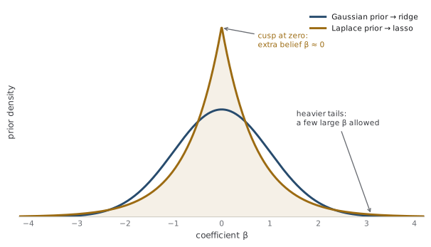
The prior view even explains why the Laplace penalty produces exact zeros while the Gaussian one does not. A Gaussian prior is flat at its peak — its slope vanishes at zero — so it exerts no pull on a coefficient that is already near zero, and the data can always nudge it a hair off. The Laplace prior has a cusp at zero: its slope does not vanish there but jumps, so it pulls with undiminished force right up to the origin, strong enough to hold a weak coefficient pinned exactly at zero. The corner of the diamond and the cusp of the Laplace density are the same fact wearing two costumes.
Note
This equivalence is why shrinkage, from the Stein surprise of Chapter 13 onward, keeps reappearing across the book. Pulling estimates toward a common center is placing a prior centered there, whether or not anyone says the word "prior." The frequentist earns lower risk by trading bias for variance (Chapter 12); the Bayesian earns the same estimator by writing down a belief. They meet at the identical formula and disagree only about the story.
A sharper question
If ridge is just a Gaussian prior, does that mean the MAP estimate is the whole Bayesian answer? No, and the gap matters. The MAP is a single point — the mode of the posterior — while the Bayesian keeps the entire posterior distribution (Chapter 9). For the lasso the difference bites hard: the posterior mean under a Laplace prior is never exactly zero, because the smooth posterior has mass on both sides of zero, so it is only the mode that lands on the axis. Lasso's celebrated sparsity is a property of MAP estimation, not of the underlying Bayesian model — full Bayesian inference with a Laplace prior gives you shrinkage but no exact zeros. The exact zero is an artifact of reporting the peak, exactly as the constraint figure warned.
References
- Hoerl, A. E., & Kennard, R. W. (1970). Ridge Regression: Biased Estimation for Nonorthogonal Problems. Technometrics.
- Tibshirani, R. (1996). Regression Shrinkage and Selection via the Lasso. Journal of the Royal Statistical Society: Series B.
Check yourself
A few questions to test the ideas from this chapter. Pick an answer to see whether it holds up.
-
Ridge and lasso start from the same least-squares fit and add a penalty on coefficient size. Holding the penalty strength fixed at some positive value, what is the essential difference in the fits they return?
The squared L2 penalty has zero slope at the origin, so it never pins a coefficient exactly at zero; the L1 penalty has a constant slope right up to zero, strong enough to hold weak coefficients there. That is why lasso does variable selection and ridge does not. -
In the budget picture, the fit is where the elliptical residual contours first touch the region of allowed coefficients. Why does this make lasso sparse but not ridge?
Sparsity comes from the geometry of the constraint region, not from the data: the diamond's corners sit on the axes and catch the ellipse there. The residual contours are the same shape in both cases; only the region differs. -
A penalized regression is exactly a MAP estimate. Under the standard Gaussian-error likelihood, which prior on the coefficients reproduces the ridge penalty, and which reproduces the lasso?
Taking minus the log of a zero-mean Gaussian density yields a sum of squares; minus the log of a Laplace density yields a sum of absolute values. The penalty strength maps to the prior width: a tighter prior means heavier shrinkage. -
You run lasso on data with several strongly correlated predictors. It keeps one of them and zeros the rest. What is the safest reading of that result?
Among collinear predictors the L1 penalty tends to keep one almost arbitrarily and drop the rest, and which one survives is sample-dependent. This instability is exactly where ridge's habit of sharing weight across the cluster is an advantage. -
Full Bayesian inference with a Laplace prior gives a posterior over the coefficients. How does its behavior at zero compare to the lasso's exact zeros?
The smooth posterior places mass on both sides of zero, so its mean misses the axis; only the mode can sit exactly at zero. Lasso is MAP estimation, and its sparsity is an artifact of keeping the peak rather than the whole distribution. -
When the true signal is spread thinly across many correlated predictors, ridge often predicts better than lasso. Why?
When the truth is dense, sparsity throws away signal; ridge's smooth shrinkage keeps all the small effects and stabilizes correlated ones. When the truth is genuinely sparse, the tradeoff reverses and lasso's selection helps. Neither dominates.