18Confidence and Credible Intervals
A point estimate answers "what is your single best guess?" and then stops, saying nothing about how far off it might be. An interval says more: it hands the reader a range of parameter values the data can live with, and it attaches a number — 95%, say — to that range. But the number means two entirely different things depending on who you ask. To a frequentist it is a property of the procedure: run the whole experiment again and again, and 95% of the intervals the recipe produces will trap the fixed unknown. To a Bayesian it is a property of this interval given a prior: 95% of the posterior probability for the parameter sits inside these endpoints. The two often land on nearly the same endpoints, which is exactly what makes them so easy to confuse.
If you take one idea from this chapter, take this: a confidence level is a promise about the long-run behavior of the interval-making rule, not a probability that the fixed parameter sits inside the one interval you are holding; a credible level is the direct probability statement instead, and it costs you a prior. And underneath both lies a single mechanical fact — an interval is a whole family of hypothesis tests read at once, which is why it tells you more than any single p-value can.
18.1Two interval philosophies
Start with the frequentist object, because it is the one people misread. Fix the unknown parameter \(\theta\) at whatever value nature chose; it is a constant, not random. You draw data, and a recipe turns that data into two numbers, a lower and an upper endpoint. Because the data is random, those endpoints are random: the interval \([L(X), U(X)]\) is a random object jiggling around from sample to sample, while \(\theta\) stays put. A confidence interval at level \(1-\alpha\) is a recipe with one guarantee — that the random interval covers the fixed target a fraction \(1-\alpha\) of the time, whatever the target happens to be (Neyman, 1937). The coverage of the recipe is that probability, \(P_\theta\big(\theta \in [L(X), U(X)]\big)\), computed over the sampling distribution of the data (Chapter 5); a valid recipe keeps it at \(1-\alpha\) for every \(\theta\), and the number \(1-\alpha\) is the recipe's confidence level. Nothing here is a statement about any single interval. The randomness is all in the endpoints, and coverage is a batting average of the procedure that made them.
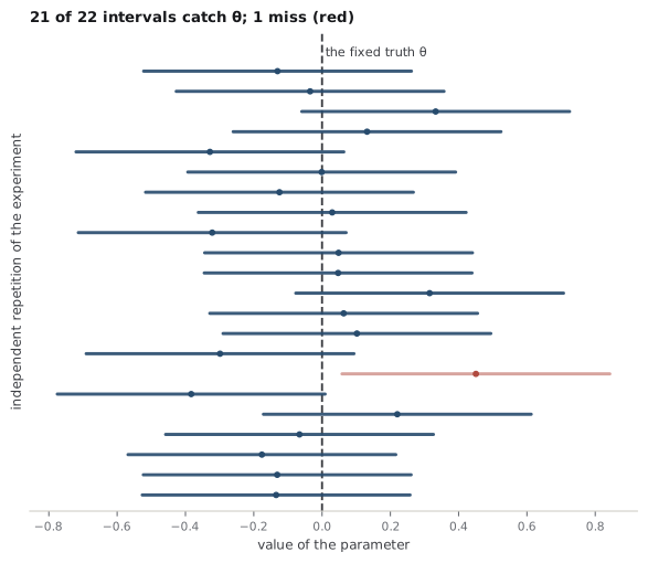
That last clause is the whole subtlety, and it is worth saying slowly.
Common trap
After you observe the data, it is tempting to read "95% confidence" as "there is a 95% probability that \(\theta\) lies in \([3.1, 4.8]\)." Under the frequentist definition this sentence is malformed. Once the data is in, both endpoints are fixed numbers and \(\theta\) is a fixed number, so \(\theta\) is either in \([3.1, 4.8]\) or it is not — the probability is \(0\) or \(1\), you just do not know which. The 95% never attached to this interval; it attached to the method that generated it. The only fully correct reading is the long-run one: "if I repeated this procedure, 95% of the intervals it produces would contain \(\theta\)." The credible interval later in this section is the object that does license the tempting sentence, and it needs a prior to do so.
A sharper question
If 95% of the intervals cover θ, and I am holding one of them, why isn't there a 95% chance mine is one of the good ones? Because "95% of intervals cover" is an average over the randomness in the data, and once you have seen your data there is no randomness left to average over — your interval is drawn, its endpoints are numbers, and \(\theta\) is a number. The 95% describes the reference set of all the intervals you might have gotten, not your position within it. There can even be recognizable features of your particular sample that make coverage higher or lower than 95% conditional on what you saw; Fisher pressed exactly this point, and it is why some statisticians condition on an ancillary statistic before quoting a number (Cox, 2006). The unconditional 95% is honest as a long-run frequency and silent about your single case.
How do you build such a recipe? The cleanest route is a pivotal quantity: a function of both the data and the parameter whose distribution does not depend on the parameter at all. The workhorse example is the standardized sample mean. If \(X_1, \dots, X_n\) are normal with unknown mean \(\mu\) and known standard deviation \(\sigma\), then
and the right-hand side knows nothing about \(\mu\) — that is what makes \(Z\) a pivot. Because its distribution is fixed, you can bracket it with fixed quantiles, \(P(-1.96 \le Z \le 1.96) = 0.95\), and then invert the inequality to isolate \(\mu\):
The endpoints \(\bar X \pm 1.96\,\sigma/\sqrt n\) are the confidence interval, and its half-width is \(1.96\) standard errors. When \(\sigma\) is unknown you swap in the sample standard deviation and the pivot becomes Student's \(t\) with \(n-1\) degrees of freedom, which widens the interval to pay for the extra thing you estimated. The pivot is the trick that turns a statement about a known distribution into a statement about an unknown parameter.
Intuition
A pivotal quantity is a rigid ruler whose markings do not shift when the parameter does. You lay it against the data, read off where the fixed 95% marks fall, and the two marks fence in every parameter value consistent with what you saw. Coverage is guaranteed because the ruler's scale — the pivot's distribution — was never allowed to depend on the thing you are measuring.
Now the Bayesian object, which starts from a different picture (Chapter 9). Treat \(\theta\) as uncertain and give it a prior; multiply by the likelihood; normalize to get the posterior, a full distribution over \(\theta\) given the data you actually saw. A credible interval at level \(1-\alpha\) is any interval holding that share of the posterior probability, and because the posterior is a distribution over the parameter, the sentence the frequentist could not say is now exactly right: \(P(\theta \in [a, b] \mid X) = 0.95\), given the prior and the data. There is no reference to repeated experiments and no long-run average; the probability is about the parameter, conditional on this one dataset. The cost is the prior — the number is only as trustworthy as the belief you fed in.
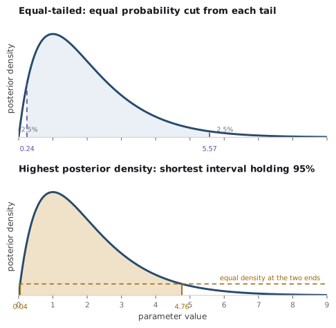
A posterior does not name a unique interval, though, so two conventions compete. The equal-tailed interval chops \(\alpha/2\) of the posterior probability off each tail, running from the \(\alpha/2\) quantile to the \(1-\alpha/2\) quantile. The highest posterior density interval, or HPD, instead collects the shortest interval that still holds \(1-\alpha\) of the mass — equivalently, every point inside it has higher posterior density than every point outside, so its two ends sit at equal density like a waterline across the distribution. On a symmetric, unimodal posterior the two agree exactly. On a skewed posterior they part ways: the HPD hugs the mode and comes out shorter, while the equal-tailed interval is stretched by the long tail it refuses to cut asymmetrically (Gelman et al., 2013).
A sharper question
When does a credible interval come out numerically equal to the confidence interval — and does that mean the distinction is just philosophy? They match in the clean cases and diverge in the interesting ones. Put a flat prior on a normal mean and the posterior is \(\mathcal{N}(\bar X, \sigma^2/n)\), whose equal-tailed 95% credible interval is \(\bar X \pm 1.96\,\sigma/\sqrt n\) — the very confidence interval from the pivot above. More generally, symmetric location problems and large samples drive the two together, and there is a whole theory of probability-matching priors chosen so that credible sets have correct frequentist coverage to high order. But the agreement is numerical, not conceptual: the same endpoints carry a statement about the procedure on one reading and a statement about the parameter on the other. And the match breaks precisely where it matters — under an informative prior, for a skewed posterior, near a hard boundary, or with small \(n\) — so treating them as interchangeable is safe only in the symmetric large-sample corner where nothing is at stake.
18.2Duality with testing
The frequentist interval and the hypothesis test (Chapter 16) are not two topics; they are one object seen from two sides. Recall that a level-\(\alpha\) test of the null \(H_0: \theta = \theta_0\) carves the data space into a rejection region and its complement, the acceptance region \(A(\theta_0)\) — the set of outcomes that do not lead you to reject \(\theta_0\). Now do this for every candidate value \(\theta_0\) at once, and after seeing data \(x\) collect the nulls that survived:
This set \(C(x)\) is a confidence set at level \(1-\alpha\), and the proof is one line: \(P_\theta(\theta \in C(X)) = P_\theta(X \in A(\theta)) = 1 - \alpha\), because the test controls its false-rejection rate at \(\alpha\) for the true \(\theta\). This is the test–interval duality: the \(1-\alpha\) confidence set is exactly the set of null values you would not reject at level \(\alpha\), and running the construction backward, any confidence procedure defines a family of tests. Inverting a test gives you an interval; inverting an interval gives you a test (Casella & Berger, 2002).
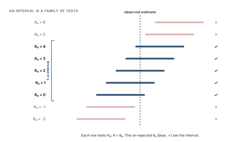
This duality is why an interval is so much more informative than a lone p-value, and the point is worth pressing.
A sharper question
What does inverting the test actually buy me over just reporting whether p < 0.05? A p-value answers one yes-or-no question about one null, usually \(\theta_0 = 0\): could this value plausibly have produced the data? The interval answers that question for every value simultaneously and hands you the full set that passes. That extra information settles the questions a bare "significant" cannot. Is the effect big enough to care about, or significant but trivially small? The interval's location tells you. How precisely did the study pin the parameter down? The interval's width tells you. And you can read the test straight off it: \(\theta_0\) lies outside the \(1-\alpha\) interval if and only if the level-\(\alpha\) test rejects \(\theta_0\), so "\(0\) is outside the 95% interval" and "\(p < 0.05\) against the null of zero" are the same statement (Chapter 17). The interval contains the p-value's verdict and adds the effect size and the precision the p-value discarded.
Note
The duality also explains why a one-sided test gives a one-sided interval. Invert a test that only rejects when the estimate is too large, and the surviving nulls form a ray \((-\infty, U(x)]\) — an upper confidence bound with no lower end. This is the natural report when only one direction is a failure: a bound on a contaminant, a floor on a reliability. The machinery is identical; you have simply put all of \(\alpha\) into one tail, which is also why the one-sided credible and confidence intervals can disagree more sharply than their two-sided cousins, since a skewed posterior treats the two directions differently.
Honesty requires naming where the frequentist construction misbehaves, because the coverage guarantee is weaker than it first sounds. Coverage is an average over the sampling distribution, and averages can hide ugly particular cases.
Common trap
A procedure with exact \(1-\alpha\) coverage can still return, on a specific dataset, an interval that is empty or one that is the entire parameter space — and both are "correct" 95% procedures. Inverting certain tests (the classic examples are ratios of normal means and parameters pinned against a physical boundary) can leave no null value un-rejected, so \(C(x)\) is empty, asserting there is no value of \(\theta\) consistent with the data even though some value generated it. Other samples reject nothing, so \(C(x)\) swallows the whole line and says nothing at all. These are not bugs in the arithmetic; they are the price of a guarantee that lives at the level of the procedure. An empty interval on your desk is a vivid reminder that "95% of intervals cover" was never a claim about the one in front of you, and it is a large part of why some analysts condition on the data's informative features, or turn to a posterior, before quoting a range (Cox, 2006).
Analogy
A confidence procedure is like a factory whose quality guarantee is "95% of the parts we ship meet spec." That is a real, checkable promise about the factory's output over the long run. It is not a promise about the single part in your hand, which either meets spec or does not; and on a bad day the factory can ship a part that is obviously broken while the 95% figure stays perfectly true. The analogy leaks in one place worth flagging: a factory could in principle inspect each part before shipping, whereas the frequentist interval refuses on principle to condition on the one dataset — which is precisely the refusal the Bayesian credible interval abandons in exchange for a prior.
References
- Casella, G., & Berger, R. L. (2002). Statistical Inference, Second Edition. Duxbury Press.
- Cox, D. R. (2006). Principles of Statistical Inference. Cambridge University Press.
- Gelman, A., Carlin, J. B., Stern, H. S., Dunson, D. B., Vehtari, A., & Rubin, D. B. (2013). Bayesian Data Analysis, Third Edition. Chapman and Hall/CRC.
- Neyman, J. (1937). Outline of a Theory of Statistical Estimation Based on the Classical Theory of Probability. Philosophical Transactions of the Royal Society A.
Check yourself
A few questions to test the ideas from this chapter. Pick an answer to see whether it holds up.
-
You compute a 95% confidence interval and get [3.1, 4.8]. Which statement is the only fully correct reading under the frequentist definition?
Coverage is a long-run property of the procedure: 95% of the random intervals it makes cover the fixed target. Once the data is in, the endpoints and the parameter are all fixed numbers, so the chance this interval contains it is 0 or 1, not 0.95. The parameter does not vary across samples (the intervals do), and an interval for a parameter is not a prediction interval for new data points. -
What property of a pivotal quantity is exactly what lets you turn it into a confidence interval with correct coverage?
A pivot mixes data and parameter into a quantity whose distribution is parameter-free, so you can bracket its fixed quantiles and solve for the parameter. Being unbiased, exactly normal, or the MLE are none of them the requirement: the standardized mean with unknown variance is not normal but a t pivot, and it still gives exact coverage because its distribution does not depend on the mean. -
By test-interval duality, the 1 minus alpha confidence set for a parameter is exactly which collection of values?
The confidence set gathers the nulls that survive testing, and its coverage follows in one line from the test's level: the true value escapes rejection with probability 1 minus alpha. Rejected values are the complement. A raw likelihood cutoff is a different (likelihood-interval) construction, and a posterior statement is the Bayesian object, which needs a prior. -
On a right-skewed posterior, how do the equal-tailed and highest posterior density (HPD) 95% credible intervals compare?
The HPD is by definition the shortest interval holding 95%, with equal density at its ends, so on a skew it hugs the mode and comes out shorter than the equal-tailed version. The two coincide only for a symmetric, unimodal posterior; there the choice does not matter, which is why the distinction only surfaces under skew. -
Inverting a certain test yields, on your particular dataset, an EMPTY 95% confidence set. What is the right conclusion?
Coverage averages over the sampling distribution, and a procedure can hit exactly 95% while occasionally emitting an empty set or the whole line on specific samples (ratios of means and boundary problems are classic cases). An empty set is not a coverage failure or a data bug; it is the vivid reminder that the 95% never described this one interval. -
Under a flat prior, the 95% credible interval for a normal mean equals the 95% confidence interval numerically. What does this coincidence establish?
Matching numbers do not merge the meanings: one interval reports the behavior of a rule over hypothetical repeats, the other a posterior probability about the parameter given this data. The agreement is special to symmetric, large-sample, flat-prior settings and breaks under informative priors, skew, boundaries, or small n, so the two are not interchangeable in general.