9The Bayesian View
A frequentist and a Bayesian look at the same coin and disagree about what is even uncertain. To the frequentist of Chapter 1, the coin's bias is a fixed number you happen not to know; all the randomness lives in the data, and a good procedure is judged by how it behaves across the samples that number could have produced. The Bayesian move is to put the uncertainty where your ignorance actually sits — on the parameter itself — and to describe that ignorance with a probability distribution. Data then has exactly one job: to reshape the distribution. This chapter is about that reshaping, and about the small miracle that, for the right pairings of belief and data, the reshaping is nothing but arithmetic.
If you take one idea from this chapter, take this: treat the unknown as random, and learning from data collapses to a single mechanical step — multiply your prior belief by what the data says, then renormalize.
9.1Belief as a distribution
Start where Chapter 1 left the parameter: a fixed feature of the world, say a coin's bias \(\theta\), that you cannot see directly. The Bayesian does not deny that \(\theta\) has some true value; the shift is epistemic. Since you are uncertain about it, you represent your uncertainty as a probability distribution over the possible values, and you update that distribution as evidence arrives. Everything follows from three objects and one rule.
The first object is the prior distribution \(p(\theta)\): a probability distribution over the parameter that encodes what you believe before seeing this data — that a manufactured coin is probably near fair, that a rate must lie in \([0,1]\), or simply that you have no idea and every value is equally plausible. The second is the likelihood \(p(x \mid \theta)\): how probable the observed data \(x\) is for each candidate value of \(\theta\), read as a function of \(\theta\) with the data held fixed. This is the same object Chapter 8 builds maximum likelihood on; here it plays the role of "what the data says." The third is the posterior distribution \(p(\theta \mid x)\): your belief about \(\theta\) after folding the data in. The rule that turns the first two into the third is Bayes' rule, and in its most useful form it reads
In words: the posterior is proportional to the prior times the likelihood. The proportionality hides a constant, and restoring it gives the full statement,
The denominator \(p(x)\) is the marginal likelihood, also called the evidence: the probability of the data averaged over every parameter value the prior allows. It does not depend on \(\theta\) — it is a fixed number whose only job is to rescale the numerator so the posterior integrates to one. That is why the proportional form carries all the action: the shape of the posterior is the product prior \(\times\) likelihood, and the evidence merely normalizes it. Computing that integral is easy in the conjugate cases below and the central difficulty of Bayesian computation everywhere else (Wasserman, 2004).
Intuition
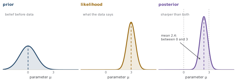
The posterior is a compromise between the prior and the likelihood, and each side pulls with a force equal to its sharpness. A confident prior and a vague likelihood land the posterior near the prior; a flat prior and a decisive likelihood hand the answer to the data. Precision, not volume, wins the argument.
Analogy
Picture the prior and the likelihood as two overlapping spotlights on a wall: the posterior is bright only where both shine. The analogy leaks in one crucial place — spotlights add their light, but Bayes' rule multiplies. A spot the prior leaves completely dark stays dark no matter how brightly the data shines on it, because anything times zero is zero. Multiplication, not addition, is what makes the next section's trap bite.
A sharper question
If two careful analysts start from different priors, they can reach different posteriors from the same data — isn't that fatal to objectivity? They can differ, but usually only when the data is thin. As evidence accumulates the likelihood grows peaked and dominates the product, so posteriors built from different reasonable priors are dragged together toward the same place — the data eventually overrules the starting point. Disagreement that survives a large sample is a signal that the priors disagreed about what is even possible, not merely about what is likely, which is exactly the failure the common trap below describes.
9.2Watching belief update
Make the machinery concrete with the cleanest conjugate pair there is, the one the widget below runs on. You are estimating a rate \(p\) — a coin's bias, a click-through rate, a cure probability. Put a Beta prior on it, \(p \sim \text{Beta}(\alpha, \beta)\), whose density is proportional to \(p^{\alpha-1}(1-p)^{\beta-1}\); the two counts \(\alpha\) and \(\beta\) act like imagined prior "successes" and "failures" that shape your starting belief. Now observe \(s\) successes and \(f\) failures. Each independent trial contributes a factor of \(p\) for a success and \(1-p\) for a failure, so the likelihood is proportional to \(p^{s}(1-p)^{f}\). Multiply, as Bayes' rule instructs:
The right-hand side is another Beta density — a \(\text{Beta}(\alpha + s,\, \beta + f)\). Updating on data did not reshape the distribution into something new; it just added your successes to \(\alpha\) and your failures to \(\beta\). Belief revision has become bookkeeping: keep two running counts and increment them.
The widget starts from a \(\text{Beta}(2, 2)\) prior — a gentle hump over \(p = \tfrac12\), mildly betting the rate is middling. Slide the success and failure counts and watch the solid posterior slide toward the observed proportion \(s/(s+f)\), marked by the vertical line, and sharpen as the counts grow. With only a handful of trials the dashed prior still visibly tugs the posterior toward the center. Pile on data and that tug fades to nothing: the posterior narrows into a spike sitting almost exactly over the data proportion, and the prior might as well not be there.
Note
The tug-of-war has an exact form. The posterior mean of a \(\text{Beta}(\alpha+s,\beta+f)\) is \(\frac{\alpha+s}{\alpha+\beta+s+f}\), which rearranges into a weighted average of the prior mean \(\frac{\alpha}{\alpha+\beta}\) and the data proportion \(\frac{s}{s+f}\), with weights \(\frac{\alpha+\beta}{\alpha+\beta+n}\) and \(\frac{n}{\alpha+\beta+n}\) for \(n = s+f\) trials. The quantity \(\alpha+\beta\) is a prior sample size: it says how many trials of imagined experience your prior is worth. Real data outvotes it as soon as \(n\) grows past it, which is the precise sense in which the data eventually dominates.
Common trap
The prior only "washes out" with more data if it grants the truth a fighting chance. Because Bayes' rule multiplies, any value the prior assigns zero probability keeps zero probability in the posterior forever — no amount of evidence can revive it. A prior that is uniform on \([0, 0.5]\) can never conclude a coin favors heads, however lopsided the flips, because it multiplied that whole region by zero at the start. A prior is a commitment about what is possible, not merely a guess about what is likely, and the possible cannot be enlarged by data.
9.3Conjugacy, and the whole posterior
The Beta-Binomial update was suspiciously tidy, and it is not a coincidence. When a prior is chosen so that the posterior lands back in the same family — Beta stays Beta — that prior is a conjugate prior for the likelihood (Chapter 4), and the update collapses to bumping a few numbers instead of recomputing an integral. This is a structural gift of the exponential family from Chapter 4, not luck distribution by distribution: every exponential-family likelihood has a matched conjugate prior, and updating simply adds the data's sufficient statistic to the prior's pseudo-counts (Diaconis & Ylvisaker, 1979). The Beta-Binomial adds successes and failures; a Gamma prior on a Poisson rate adds the event count and the exposure and stays Gamma; a Normal prior on a normal mean stays Normal, its precision the sum of the prior and data precisions — the very update drawn in the first figure. Sufficiency, conjugacy, and clean updating are one idea seen from three doorways, exactly as Chapter 4 promised.
Set the prior to flat and the Bayesian and frequentist pictures nearly touch. With a uniform prior the posterior is proportional to the likelihood alone, so its peak — the single most probable parameter value, the maximum a posteriori or MAP estimate — sits exactly at the maximum-likelihood estimate of Chapter 8. In this loose sense the MLE is "the Bayesian answer under a flat prior, then thrown away except for its peak." And that discarding is the real difference between the two stances. A frequentist reports a point — the MLE and a standard error around it. A Bayesian reports the whole posterior distribution, a full curve of relative plausibility, and any single number you might quote from it is a lossy summary of that curve (Gelman et al., 2013).
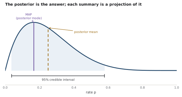
Which number you report is a decision, and different summaries answer different questions. The MAP gives the single likeliest value; the posterior mean minimizes expected squared error and, for a skewed posterior, differs from the mode; the posterior median splits the probability in half. For an interval, you quote a credible interval — a range holding a stated share of the posterior probability, say 95%. That phrase means what a newcomer hopes an interval means: given this prior and this data, there is a 95% probability the parameter lies inside. It is tempting to read a frequentist confidence interval the same way, which brings us to the sharpest trap in the chapter.
Common trap
A credible interval is not a confidence interval, even when they happen to coincide numerically. A 95% credible interval makes a probability statement about the parameter: it is 95% probable to be in here. A 95% confidence interval makes a probability statement about the procedure: intervals built this way trap the true value 95% of the time across repeated samples, which says nothing about whether this one interval does. The guarantees live in different places — one in your posterior, the other in the sampling distribution — and Chapter 18 is devoted to keeping them apart.
A sharper question
If the MAP is just the MLE under a flat prior, is Bayesian inference merely maximum likelihood with extra steps? No, and the figure shows why: the point is that you keep the entire posterior rather than its peak. That buys three things a point estimate cannot. The spread of the posterior is your calibrated uncertainty, delivered without asymptotic approximation. The mean and the mode part ways whenever the posterior is skewed, so "the estimate" is genuinely ambiguous until you say which summary you mean. And a flat prior is often not innocent — it can be improper, and worse, "flat" in one parameterization is curved in another, so even the MAP quietly depends on a modeling choice the MLE pretends it has escaped.
Note
This chapter's machinery reappears wearing a penalty. A regularized estimate — ridge, lasso — is precisely a MAP estimate under a prior that pulls coefficients toward zero: a Normal prior yields the ridge penalty, a Laplace prior the lasso. "Penalize large coefficients" and "believe coefficients are probably small" are the same sentence in two dialects, which is the whole argument of Chapter 14.
Seen this way, the Bayesian view is less a rival to estimation than a different accounting of it. Where the frequentist grades a procedure by its behavior over hypothetical samples, the Bayesian carries uncertainty in the answer itself, as a distribution that data sharpens. The two agree in the large-sample limit, where the likelihood swamps any reasonable prior and the posterior goes normal around the MLE — a convergence Chapter 19 makes precise. What the Bayesian keeps, and the point estimate forfeits, is the shape of the doubt.
References
- Diaconis, P., & Ylvisaker, D. (1979). Conjugate Priors for Exponential Families. The Annals of Statistics.
- Gelman, A., Carlin, J. B., Stern, H. S., Dunson, D. B., Vehtari, A., & Rubin, D. B. (2013). Bayesian Data Analysis, Third Edition. Chapman and Hall/CRC.
- Wasserman, L. (2004). All of Statistics: A Concise Course in Statistical Inference. Springer.
Check yourself
A few questions to test the ideas from this chapter. Pick an answer to see whether it holds up.
-
In the full statement of Bayes' rule, the denominator is the marginal likelihood p(x), the probability of the data averaged over the prior. What is its role in shaping the posterior?
The evidence does not depend on the parameter, so it cannot reweight one value against another or 'move' belief — that work is done entirely by the numerator, prior times likelihood. It is a pure normalizing constant. Its one further use is across models rather than within one: comparing the evidence of competing models is the basis of Bayes factors. -
You report a 95% credible interval for a parameter. How does its meaning differ from a 95% confidence interval?
The guarantees live in different places: the credible interval's probability is about the parameter given your posterior, while the confidence interval's is about the method across repeated samples and says nothing about whether this particular interval traps the truth. The last option swaps the two, the classic misreading Chapter 18 is built to prevent. Numerically they can even coincide while meaning different things. -
A Beta prior on a rate meets Bernoulli data and yields a Beta posterior; a Gamma prior on a Poisson rate stays Gamma. Why do such conjugate pairs exist so reliably?
Conjugacy is the exponential-family structure of Chapter 4 seen in Bayesian dress: because the parameter meets the data only through a sufficient statistic in the exponent, updating just increments the prior's counts. It has nothing to do with the prior being flat, and it is a structural guarantee, not a lucky coincidence for a handful of named pairs. -
Under a flat prior, the MAP estimate coincides with the maximum-likelihood estimate. Does that make Bayesian inference just maximum likelihood with extra bookkeeping?
Matching the MLE at the peak is not the same as carrying no more information: the posterior's whole shape is the uncertainty, the mean parts from the mode whenever it is skewed, and 'flat' is not innocent — it can be improper and is not invariant to reparameterization. The MAP and MLE do coincide under a flat prior, so the option claiming they disagree is simply wrong. -
An analyst uses a prior that is uniform on [0, 0.5] for a coin's bias p, then collects flips that are overwhelmingly heads. What does the posterior conclude?
A prior is a statement about what is possible, not merely likely: multiplying a region by zero leaves it zero forever, so the posterior piles up against the 0.5 boundary but can never cross it, no matter how lopsided the flips. The 'data always washes out the prior' rule holds only when the prior grants the truth positive probability, which this one refuses to do. -
With a Beta(alpha, beta) prior and n = s + f observed trials, the posterior mean is a weighted average of the prior mean and the data proportion. What plays the role of the prior's weight?
The posterior mean weights the prior mean by (alpha + beta) / (alpha + beta + n) and the data proportion by n / (alpha + beta + n), so alpha + beta behaves like a count of imagined prior trials. Real data overrules it as soon as n exceeds it — the exact sense in which belief starts near the prior and ends near the data.