Chapter 5

5Convergence and the Limit Theorems

Two theorems quietly run all of statistics, and both are statements about what happens to an average as you collect more data. The first, the law of large numbers, says the average settles down: pile up enough observations and their mean stops wandering and locks onto the true mean. The second, the central limit theorem, says exactly how the average wiggles on its way there: rescaled the right way, that wiggle is a bell curve, no matter what the raw data looks like. Together they answer the two questions that make estimation possible at all — does averaging converge on the truth? and how far off is it likely to be? — and they are why the normal distribution shows up everywhere and why a "standard error" means anything.

Before either theorem can even be stated, though, you need to say what "the average converges" means, because a sequence of random quantities can approach a limit in more than one sense. So we start there.

5.1Modes of convergence

A number either converges or it does not. A sequence of random variables $X_1, X_2, \dots$ is trickier, because each $X_n$ is a whole distribution, not a point. There turn out to be three useful senses in which such a sequence can approach a limit, and they make genuinely different promises.

Convergence in probability is the workhorse. We say $X_n \to X$ in probability, written $X_n \xrightarrow{p} X$, if for every tolerance $\varepsilon > 0$, $$\mathbb{P}\big(|X_n - X| > \varepsilon\big) \to 0 \quad \text{as } n \to \infty.$$ Read it literally: pick any margin you like, and the chance of $X_n$ being outside that margin eventually shrinks to nothing. It does not forbid $X_n$ from occasionally leaping far away — it only demands that such leaps become rarer and rarer. This is the mode that defines consistency of an estimator (Chapter 6): getting the right answer with high probability once you have enough data.

Almost sure convergence is stronger. We say $X_n \to X$ almost surely, written $X_n \xrightarrow{a.s.} X$, if $$\mathbb{P}\Big(\lim_{n\to\infty} X_n = X\Big) = 1.$$ Here the entire path $X_1, X_2, \dots$ settles down: with probability one, the sequence you actually observe converges in the ordinary calculus sense. Convergence in probability lets the sequence keep flickering outside the margin forever as long as it does so ever more rarely; almost sure convergence says the flickering stops.

Convergence in distribution is the weakest, and it is about shape, not location. We say $X_n \to X$ in distribution, written $X_n \xrightarrow{d} X$, if the cumulative distribution functions converge, $$F_n(x) \to F(x) \quad \text{at every } x \text{ where } F \text{ is continuous.}$$ Nothing here says $X_n$ itself lands anywhere near $X$ — only that the distribution of $X_n$ comes to look like the distribution of $X$. That is precisely the promise the central limit theorem cashes in.

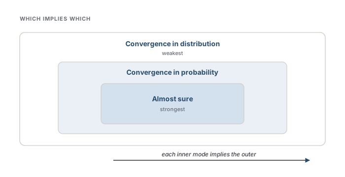
The three are nested, strongest to weakest: $$X_n \xrightarrow{a.s.} X \;\;\Longrightarrow\;\; X_n \xrightarrow{p} X \;\;\Longrightarrow\;\; X_n \xrightarrow{d} X.$$ The arrows run one way only. A sequence can converge in distribution without ever settling on a value, and converge in probability without its path ever quieting down.

Figure 5.1The modes nest. Almost sure convergence sits inside convergence in probability, which sits inside convergence in distribution: each inner mode implies every outer one, and none of the reverse arrows hold in general. The theorems of this chapter live at two of these rings — the law of large numbers in the inner two, the central limit theorem in the outermost.

Intuition

Three questions of increasing strictness. In distribution: does $X_n$ come to have the right shape? In probability: does $X_n$ come to sit near the right value? Almost surely: does the sequence you actually watch quiet down and stay put? Each yes is harder to earn than the last.

Note

There is one useful partial converse. If the limit is a constant $c$ rather than a genuine random variable, then $X_n \xrightarrow{d} c$ implies $X_n \xrightarrow{p} c$. Converging in distribution to a fixed point leaves nowhere for the mass to hide, so the two coincide. This is why the law of large numbers, whose limit is the constant $\mu$, can be stated in either mode without fuss.

A sharper question

If almost sure convergence is strictly stronger, why not always demand it? Because in-probability results are usually all you need to justify a method and are far easier to prove, while almost sure statements often require more assumptions and heavier machinery for no extra practical payoff. Consistency, standard errors, and confidence intervals all rest on convergence in probability and in distribution. Almost sure convergence is the sharper mathematical object; convergence in probability is the one you reach for.

5.2The law of large numbers

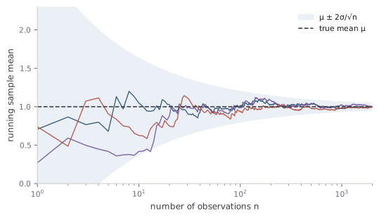
Now fix an actual quantity of interest. Let $X_1, \dots, X_n$ be independent draws from a distribution with mean $\mu$ and finite variance $\sigma^2$, and form the sample mean $$\bar X_n = \frac{1}{n}\sum_{i=1}^n X_i.$$ The law of large numbers (LLN) says this average converges to $\mu$: as $n$ grows, $\bar X_n \to \mu$. That is the whole reason estimation by averaging works. The empirical average of your data is not just a plausible guess at the mean — it is guaranteed to close in on it.

The law comes in two strengths, matching two of the modes above. The weak law says $\bar X_n \xrightarrow{p} \mu$: the average converges in probability. The strong law says $\bar X_n \xrightarrow{a.s.} \mu$: the whole sequence of running averages settles down and stays. The strong law is the more satisfying statement and needs only that the mean exists; the weak law is the one you actually invoke, because in-probability convergence is what consistency arguments require.

You can feel where the weak law comes from in one line. The variance of the sample mean is $\operatorname{Var}(\bar X_n) = \sigma^2 / n$, which goes to zero. An estimator whose bias is zero and whose variance vanishes cannot help but concentrate on its target — that is Chebyshev's inequality turning a shrinking variance directly into a shrinking probability of being far off. The average settles because its spread is being squeezed out at rate $1/n$.

A line plot of the running sample mean against the number of observations n on a logarithmic horizontal axis. Three jagged sample paths start far apart at small n and all funnel inward toward a horizontal dashed line marking the true mean mu. A shaded band around mu narrows from left to right, tracking the one-over-square-root-n shrinkage of the fluctuations. — Figure 5.2The average stops moving. Three independent streams of draws, each shown as its running mean, start scattered and converge on the true mean mu as n grows. The shaded band narrows like one over the square root of n — the fluctuations do not vanish suddenly, they are gradually squeezed. That rate is exactly what the next theorem makes precise.

Intuition

The law of large numbers says the average stops moving. Early on, each new observation can swing the running mean around; but every later point carries weight only $1/n$, so the average grows sluggish and eventually parks itself on $\mu$.

Analogy

Filling a bathtub with cups of water of slightly different sizes. The first few cups make the level jump, but once the tub is nearly full, one more cup barely moves it. The average cup size is the water level, and it stabilizes not because the cups stop varying but because each one matters less. The analogy leaks in that a tub has a fixed capacity, while the sample mean has no ceiling — it stabilizes purely because of the $1/n$ weighting, not because it runs out of room.

Common trap

The law of large numbers is about the average, not about individual draws, and it has no memory. A run of low values does not make high values "due" to balance them out — the average dilutes the imbalance by collecting more terms, it does not reverse it. Believing otherwise is the gambler's fallacy.

The law tells you the average lands on $\mu$, but it is silent on how far off you are at any finite $n$, and that gap is where all the practical work happens. Answering it needs a finer instrument than "the variance goes to zero."

5.3The central limit theorem

The law of large numbers says $\bar X_n - \mu \to 0$, so if you want to see the fluctuation rather than watch it vanish, you have to magnify it as it shrinks. The right magnification is $\sqrt{n}$, and blowing the difference up by that factor reveals a startlingly universal shape. The central limit theorem (CLT) states that for independent draws with mean $\mu$ and finite variance $\sigma^2$, $$\sqrt{n}\,\big(\bar X_n - \mu\big) \;\xrightarrow{d}\; \mathcal{N}\!\big(0, \sigma^2\big).$$ The standardized average converges in distribution to a normal with variance $\sigma^2$ — and the source distribution has vanished from the right-hand side entirely. Skewed, discrete, heavy-shouldered, bimodal: whatever the $X_i$ look like, the rescaled mean forgets it. Only the mean and variance survive.

Equivalently, and this is the form you will use, the sample mean is approximately normal around the truth, $$\bar X_n \;\approx\; \mathcal{N}\!\Big(\mu, \;\frac{\sigma^2}{n}\Big),$$ with spread $\sigma/\sqrt{n}$. That spread is the standard error: the standard deviation of an estimator's own sampling distribution, the typical distance between your estimate and its target. The CLT is what lets you attach a $\sigma/\sqrt{n}$ to an average and call it a margin of error.

Slide the sample size up in the panel below and watch it happen. The source distribution on offer is visibly lopsided — nothing like a bell. At $n = 1$, the sampling distribution of the mean (the histogram you get by drawing a sample, averaging it, and repeating many times) is just as lopsided, because a mean of one number is that number. Push $n$ higher and the histogram of sample means pulls itself upright, sheds its skew, and slides under the normal overlay, even though every underlying draw still comes from the same skewed source.

Intuition

The law of large numbers tells you where the average goes; the central limit theorem tells you how it wiggles on the way. The wiggle shrinks like $1/\sqrt{n}$, and once you rescale to hold that shrinkage constant, the wiggle is always the same bell.

Common trap

The CLT is a statement about the distribution of the standardized mean, not about the distribution of the raw data. Averaging thousands of skewed observations does not make the observations look normal — they keep their skew forever. It is $\bar X_n$, the average, whose sampling distribution turns normal. Confusing the two leads people to expect their histogram of raw data to bell out as they collect more, which it never does.

Common trap

"Use the normal approximation once $n \geq 30$" is a rule of thumb, not a theorem. How fast the sampling distribution becomes normal depends on the source: a mildly skewed distribution is nearly normal by $n = 10$, while a severely skewed or heavy-tailed one may need hundreds of samples. The theorem promises convergence, not a speed; $n = 30$ is a folk shorthand that the widget above will happily violate if you pick a skewed enough source.

A sharper question

The CLT needs finite variance. What breaks without it? Everything. If the $X_i$ have infinite variance — heavy tails like a Cauchy distribution, where extreme values are common enough that $\sigma^2$ diverges — then no single giant observation ever gets diluted by its neighbors, and the $\sqrt{n}$ rescaling is simply the wrong magnification. The sample mean of Cauchy draws does not concentrate at all; astonishingly, $\bar X_n$ has the same distribution as a single draw, no matter how large $n$ is. Averaging buys you nothing. Such sums have their own limit laws (the stable distributions), but the normal is not among them. Finite variance is the price of admission to the bell.

Why does this one theorem matter so much? Because it is the engine underneath inference. Standard errors, the $\pm$ you put on an estimate, are CLT statements. Confidence intervals (Chapter 18) are built by inverting the normal approximation to the sampling distribution. And the reason maximum likelihood is asymptotically efficient (Chapter 19) — the reason it hits the smallest possible variance as data grows — is that the maximum likelihood estimator is itself asymptotically normal, with the CLT operating on the likelihood's score. The normal distribution is not everywhere by coincidence. It is everywhere because almost every estimate you will ever compute is, at bottom, an average, and the CLT says averages become normal.

Check yourself

A few questions to test the ideas from this chapter. Pick an answer to see whether it holds up.

Which chain correctly orders the three modes of convergence from strongest to weakest?
A researcher averages 10,000 draws from a strongly right-skewed distribution and is puzzled that the histogram of the raw observations is still skewed. What is the error?
Two analysts use the normal approximation for a sample mean at n = 30. One's source is mildly skewed, the other's severely skewed. What does the CLT actually guarantee?
Why does the central limit theorem fail for independent draws from a Cauchy distribution?
The weak law of large numbers can be read straight off one fact about the sample mean. Which fact?
Convergence in distribution is generally weaker than convergence in probability, yet they coincide in one important case. Which?