6What Makes a Good Estimator
An estimator is a rule, not a number. You feed it a dataset and it hands back a guess; feed it a different dataset drawn from the same world and it hands back a different guess. So the question "is this a good estimator?" cannot be answered by staring at the one number it gave you this time — a broken clock also produces a number, and even a superb rule will miss on some unlucky sample. What you can judge is the rule: the whole cloud of answers it would produce across every dataset the truth could have handed you. That cloud is the estimator's sampling distribution, and this chapter is about reading it.
If you take one idea from this chapter, take this: you never grade an estimate, you grade the rule — by the shape of the sampling distribution it produces across all the samples it could see.
That shift, from scoring a number to scoring a distribution, is the move that opens Part II. It also means every quality we care about is a feature of that distribution: where it sits relative to the truth, how tightly it clusters, and whether it collapses onto the truth as data accumulates. Three numbers capture the first two, and one limiting guarantee captures the third.
6.1The three summary numbers
Fix the quantity you want to estimate — call it \(\theta\), the estimand — and a rule \(\hat\theta\) that turns data into a guess for it. Because the data is random, \(\hat\theta\) is a random variable with a distribution of its own. You summarize that distribution with three numbers, and the first two answer the two most basic questions you could ask of a cloud of guesses: where is it centered, and how spread out is it?
The bias is how far the rule lands from the truth on average — the gap between the estimator's mean and the estimand:
A rule whose bias is zero for every possible value of \(\theta\) is called unbiased: run it over and over on fresh data and its guesses average out exactly to the truth. The variance is the second number — how much the guesses jitter around their own average, \(\operatorname{Var}(\hat\theta) = \mathbb{E}\big[(\hat\theta - \mathbb{E}[\hat\theta])^2\big]\) — and its square root, the standard error, is the spread in the estimator's own units. Bias is aim; variance is steadiness.
Neither number alone tells you how wrong the rule typically is, because being off-center and being jittery are both ways to miss. The third number folds them into one, by averaging the squared distance from the truth over the sampling distribution — the mean squared error:
The split is exact: add and subtract \(\mathbb{E}[\hat\theta]\) inside the square, expand, and the cross term vanishes. Total error is squared bias plus variance — miss the center or spray your shots, and either way you pay.
Intuition
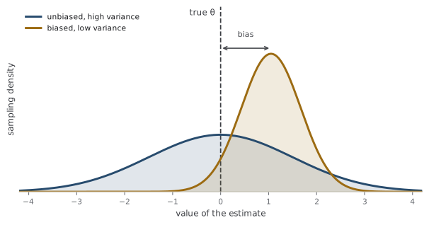
Bias, variance, and MSE describe a cloud, not a point. Bias is where the cloud's center sits relative to the bullseye, variance is how loose the cloud is, and MSE is the average squared distance from the bullseye to a dart in it. You are grading the thrower, not the throw.
The dartboard picture — a cluster that can be off-center, spread out, or both — is the same one that runs the bias-variance tradeoff in Chapter 12. Here the point is narrower and worth stating flatly: because MSE adds squared bias to variance, the unbiased rule is usually not the one with the lowest error. Zeroing the bias term does nothing to stop the variance term from being large, and often you can trade a pinch of bias for a larger cut in variance and drive MSE down.
A concrete case makes it vivid. To estimate the variance \(\sigma^2\) of a normal population from \(n\) observations, you sum the squared deviations from the sample mean and divide by something. Divide by \(n-1\) and you get the textbook unbiased estimator. Divide by \(n\) instead — the maximum-likelihood choice (Chapter 8) — and you get a biased estimator that nonetheless has smaller MSE. Push further: dividing by \(n+1\) minimizes the MSE among all these, and it is more biased still. The estimator everyone calls "correct" is not the one that is typically closest to the truth (Cox, 2006).
Common trap
Unbiased does not mean good. An unbiased rule can have enormous variance, and then it is unbiased and useless — reliably right on average while being wildly wrong on any single sample. Worse, unbiasedness can force an absurd answer: the only unbiased estimator of \(e^{-2\lambda}\) from a single Poisson\((\lambda)\) count is \((-1)^{X}\), which reports \(+1\) or \(-1\) for a quantity that must lie in \((0,1)\). Being centered on the truth on average is a property of the rule, not a promise about the estimate in your hands.
A sharper question
If lower MSE is what I want, why does anyone insist on unbiasedness at all? Partly history and partly convenience: unbiasedness is easy to check, it composes nicely under averaging, and combined with a separate demand for minimum variance it singles out a unique "best unbiased" estimator with a clean theory (the Cramér–Rao bound and the information geometry behind it are Chapter 7). But that theory answers "best among unbiased rules," which is a smaller question than "best rule." The moment you let a little bias in, you can often beat every unbiased estimator on MSE — which is the whole argument of Part IV.
6.2Consistency: getting it right with enough data
Bias, variance, and MSE grade a rule at a fixed sample size. A different question asks what happens as the data piles up: does the rule home in on the truth, or can it stay stubbornly wrong no matter how much you feed it? The bare-minimum guarantee is consistency — the estimator converges to the estimand as \(n\) grows. Made precise, \(\hat\theta_n\) is consistent for \(\theta\) if it converges in probability: for any tolerance \(\varepsilon > 0\), the chance of missing by more than \(\varepsilon\) shrinks to zero,
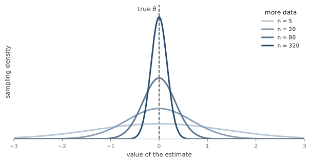
You have already met the engine that makes this happen. The law of large numbers (Chapter 5) says the sample mean converges to the true mean, so the most basic estimator there is — average your data to estimate a population average — is consistent for free (Wasserman, 2004). Consistency is the sampling distribution collapsing onto a spike at \(\theta\): its spread vanishes and its center arrives at the truth, so eventually all of its mass sits in any window you draw around \(\theta\).
Analogy
Consistency is a camera pulling into focus. A blurry photo can still be aimed at the right subject; as you turn the focus ring the blur tightens onto it. The analogy leaks in the direction of the promise: focusing is something you do in finite time, while consistency is only a statement about the limit — it guarantees the picture sharpens eventually, not that it is sharp at the sample size you actually have.
Consistency is genuinely a floor, not a certificate of quality. A consistent rule can be badly biased and jittery at every sample size you will ever collect, and only redeem itself in a limit you never reach. Two consistent estimators of the same \(\theta\) can concentrate at wildly different speeds, and the slow one may be worthless in practice. So consistency is the property you demand before anything else — a rule that does not converge to the truth even with infinite data is disqualified — but clearing that bar is the beginning of the comparison, not the end of it.
Common trap
Consistency and unbiasedness are different properties, and neither implies the other. The divide-by-\(n\) variance estimator is biased at every finite \(n\) yet perfectly consistent — its bias shrinks toward zero as the sample grows. Going the other way, "just report \(X_1\) and ignore the rest of the data" is an unbiased estimator of the mean that is hopelessly inconsistent: its sampling distribution never narrows, because it always throws away all but one observation. Unbiasedness is about the center of the cloud at one \(n\); consistency is about the cloud shrinking to a point as \(n\) grows.
A sharper question
If consistency only promises something in the limit, does it tell me anything about the finite sample I actually have? Not by itself — which is exactly why it is the floor and not the whole story. What you really want to know is how fast the sampling distribution concentrates: the typical estimator shrinks its standard error like \(1/\sqrt{n}\), and the constant out front is what separates a good rule from a merely-consistent one. Pinning down that rate, and the smallest it can possibly be, is where Fisher information and the Cramér–Rao bound come in (Chapter 7), and why maximum likelihood is asymptotically hard to beat (Chapters 8 and 19).
With these tools in hand you can finally say what "good" means and start comparing rules honestly. Bias, variance, and MSE score a rule at your sample size; consistency screens out the rules that never arrive. What none of them settles is how to score being wrong in the first place — MSE quietly assumed squared error, and other losses tell different stories. That choice, and the risk it defines, is Part III; the tradeoff between the bias and variance terms, only introduced here, is the heart of Chapter 12.
References
- Cox, D. R. (2006). Principles of Statistical Inference. Cambridge University Press.
- Wasserman, L. (2004). All of Statistics: A Concise Course in Statistical Inference. Springer.
Check yourself
A few questions to test the ideas from this chapter. Pick an answer to see whether it holds up.
-
You compute an estimate and it happens to equal the true parameter exactly. What does this tell you about the estimator you used?
Bias, variance, and consistency are all features of the rule's sampling distribution across every dataset it could see, not of one realized number. A single hit is consistent with a wildly biased or high-variance rule, just as a stopped clock is right twice a day. -
For a normal population variance, dividing the sum of squared deviations by n minus 1 is unbiased, while dividing by n is biased. Which statement is correct?
Because MSE is squared bias plus variance, the unbiased choice need not minimize it. Dividing by n lowers the variance term more than the bias term costs; pushing to n plus 1 minimizes MSE outright. MSE is defined for any estimator, biased or not. -
In what sense can an unbiased estimator still be a poor choice?
Unbiasedness constrains only the center of the sampling distribution, not its spread, so an unbiased rule can be uselessly noisy. Unbiasedness neither forces nor forbids consistency, and it does not by itself decay with n — those distractors confuse independent properties. -
Consider the rule 'estimate the population mean by reporting only the first observation and discarding the rest.' How does it behave?
A single draw has the population mean as its expectation, so the rule is unbiased; but it ignores the growing sample, so its variance never falls and it never concentrates on the truth. This is the cleanest proof that unbiasedness and consistency are independent. -
An estimator is proven consistent. What does this guarantee about its performance at the sample size you actually have?
Consistency is an asymptotic promise: the distribution collapses onto the truth eventually, saying nothing about a fixed n. Two consistent estimators can concentrate at very different rates, which is why the 1/sqrt(n) rate and its optimal constant (Chapters 7 and 19) are what actually separate good rules from merely-consistent ones.